A possible link between General Relativity and Quantum Mechanics.
1. Introduction
Anyone first encountering quantum theory is puzzled by the fact that no ontological explanation to the quantum world is given. This article shows that quantum mechanics follows naturally if the metrics of spacetime oscillate at very high frequencies. It appears that this could explain the particle-wave duality and help resolve other quantum theoretical puzzles, for example the measurement problem. It is shown that oscillating metrics treated in General Relativity (GR) naturally leads to Quantum Mechanics (QM) if a particle always is accompanied by oscillation of the spacetime metrics at the Compton frequency. In this view the quantum mechanical wave functions are modulations of this Compton "carrier" oscillation of the spacetime metrics. I derive the de Broglie matter-wave, and the de Broglie/Bohm "pilot wave" momentum relation. The Schrödinger equation is derived directly from the GR line element assuming that the metrics oscillate. This solution also models quantum jumps as a well-defined dynamic process. A detailed physical explanation for the double slit particle interference is also given.
A new cosmological model by which the universe evolves via incremental scale expansion of all four spacetime metrics (Masreliez, 1999) provided the motivation for considering oscillating spacetime metrics as a possible explanation for quantum mechanics.This incremental expansion mode is required to preserve equivalence between all locations in space and time. Regardless of the viability of this new cosmological model the main objective of the paper is to show that the quantum world might result from oscillating spacetime metrics.
2. The modulated line element and the matter-wave
The Minkowski line element is:

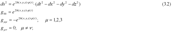
Consider the possibility that the metrics might oscillate as modeled by the line element:

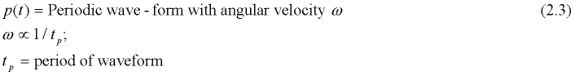
Assume a periodic function, p(t):
In particular with p(t)=C·cos(w t)=Re{C exp(-i w t}). C = constant:

In the following I will omit the label Re{ }. The use of a complex number in the exponent is to be interpreted as the real part, for example i·exp(-iw t) means sin(w t).
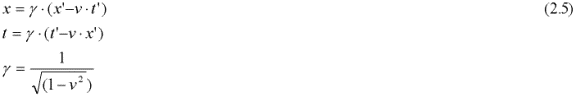
Motion of a spatially confined region with the line element (2.4) at the constant velocity v in the x direction is modeled by the Lorentz transformation:
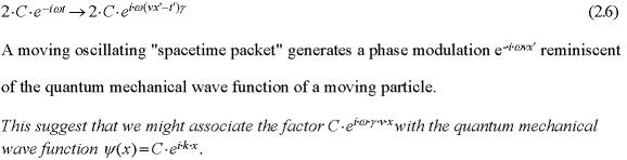
The modulating part of the exponent in the metric then becomes:
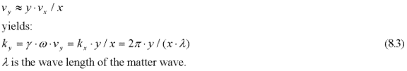
The wave number is:

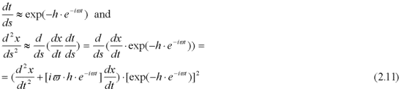
Thus, motion of a locally confined spatial region with oscillating metrics has the effect of increasing the excitation frequency and spatially modulating the phase of the excitation. It appears that this spatial modulation could be related to the quantum mechanical wave function. The relationship between the momentum and the wave number is:

This relation suggests that every particle might be associated with a metric excitation frequency that corresponds to its energy as given by (2.8), i.e. the relativistic Compton frequency.Motion causes this oscillation to be "phase modulated" in the form of a spatial wave, exp(ikx), modulating the Compton oscillation.This could be the de Broglie matter-wave. Thus, if a Compton oscillation accompanies each particle as modeled by (2.4) it will in motion create a de Broglie type spatial modulation of the metrics. In this interpretation the quantum mechanical matter-wave is a spatial wave pattern in the metrics of spacetime formed by a relativistic effect due to time dilation according to (2.6). The very high Compton frequency corresponding to the particle matter energy makes this small relativistic temporal effect significant even at relatively low velocities. With this interpretation the matter-wave is a purely relativistic phenomenon generated by motion.
To explore the possible connection between GR and QM a bit further, consider the line element:

Here the possibly of complex valued wave function h models both amplitude and phase modulation of the Compton oscillation. The geodesic equation of GR for motion in the x-direction at low velocities becomes:

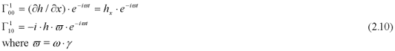
The two Christoffel symbols (see section 3) corresponding to the line element (2.4) are:
Since all velocities are small we have from the line element:
The geodesic equation becomes:

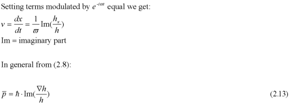
Relation (2.13) is de the de Broglie/Bohm [Bohm, 1952] momentum relation, i.e. the pilot wave guiding function, if the function h(x,y,z), which modulates the Compton oscillation, is proportional to the quantum mechanical wave function. This shows that De Broglie and Bohm's momentum relation follows directly from the geodesic equation of GR if the spacetime metrics of a particle oscillate at the Compton frequency. Thus , the previously mysterious guiding "pilot" function finds its physical explanation if a particle is accompanied by oscillation of the spacetime metrics at the Compton frequency.
3. Deriving the wave equation from General Relativity
Einstein's GR equations are:

As usual Gμν is Einstein's tensor, Rμν is the Ricci tensor, gμν the metric tensor. K is Einstein's constant and Tμν is the energy-momentum tensor. These ten equations reduce to four equations if the matrix gμν is diagonal.
Consider the line element:
The Ricci tensor is:
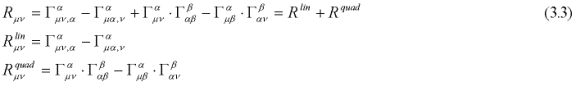
where the Christoffel symbols are:

Einstein's summation convention for repeated indices applies and all Christoffel symbols contain first derivatives of the metric as indicated by the index following the comma.
The first two terms in (3.3) are linear in the second derivatives of h(x,y,z)p(t) and will average to zero assuming that the both p(t) and its time derivatives average to zero. However, the amplitude could be large if the frequency is high. The last two terms, which are quadratic on the derivatives of the metrics, typically do not average to zero. I will treat these two contributions separately.
The contributions from the two linear terms are:


The Ricci scalar based on the linear terms in (3.3) is given by:

If p(t) is a sinusoidal excitation, setting the expression inside the bracket equal to zero results in a three-dimensional wave equation expressing resonating spatial metrics in response to the vibrating scale excitation.
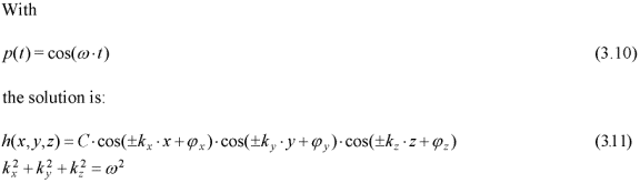
This is a family of three-dimensional standing waves, which might be viewed as the superposition of separate wave solutions traveling at the speed of light along the positive and negative coordinate axes.
The contribution to the Ricci scalar from the two last terms in relation (3.3) typically does not average to zero. These terms contain "real" energy density. However, the linear and quadratic parts of the Ricci scalar can be treated separately due to their different characters. Setting relation (3.9) equal to zero yields a relativistic wave equation, which in the special case of the modulated Minkowski metric takes the form.

The wave solution h(x,y,z) is interpreted as an amplitude and phase modulation of a high frequency carrier oscillation p(t).The remaining quadratic part Rquad of the Ricci tensor could generate a particle's matter energy. The energy density is proportional K·(C·ω)2. If the diameter of the particle is in the order of 1/ω the energy is proportional to K·C2/ ω.Setting this equal to ħ·ω the oscillation amplitude becomes:

Where Lpl is the Planck length.
For the electron C is in the order of 5·10-23.Since the amplitude of the terms in Rlin are proportional to C and the magnitude of the contribution from the terms in Rquad proportional to C2, it is not unreasonable that Rlin should equal zero, since in general relativity the gravitational field in vacuum is given by R=0.
I therefore make the following proposition:
The linear contribution to the Ricci scalar from the oscillating metrics that create a particle's rest mass energy equals zero.
The proposition above might seemed grasped out of thin air. However, the objective of this paper is not to demonstrate that the proposition holds true, but merely to show that it would provide a physical explanation to the quantum world.
Also, note that the second derivatives of the complex factor in the exponent that models the metric appear in the linear wave equation (3.12). This justifies the use of a complex exponent to express amplitude and phase modulation. Replacing the complex modulation with a superposition of cosine and sine terms will carry over to (3.12) since this equation is linear. However, this does not apply to the contribution from Rquad, which creates the rest mass energy and is non-linear.
4. The approach of Louis de Broglie and David Bohm.
Over the years several attempts have been made to explain QM. Louis de Broglie suggested at the Solvay conference in 1927 that a particle might be guided by a "pilot wave" directly related to the wave function. At this meeting he was challenged by Wolfgang Pauli to explain what happens to the pilot wave at scattering, which causes a single wave function to split up into a superposition of many different components. The single pilot wave corresponding to this superposed wave function cannot explain the different possible trajectories taken by the scattered particle. David Bohm, who independently revived De Broglie's idea, countered this challenge by speculating that decoherence quickly occurs between the different branches of the scattered wave function and that the scattered particle selects only one of the possible branches leaving the other branches "empty". The validity of this explanation is supported by our interpretation where scattered contributions to the wave function at difference energies are uncorrelated due to their different carrier frequencies. The various possible trajectories appear as different solutions to the geodesic equation, one for each carrier frequency (see further below). After scattering, the particle will take one of several possible trajectories corresponding to its energy.
David Bohm further developed de Broglie's proposal in his hidden variable theory of 1952-1954 [Bohm, 1952 and 1954]. He was able to show that QM may be developed in a straightforward manner based on the assumption that there exists in Nature a "quantum potential" of the form:
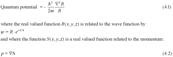
From relation (3.12) we have:

This is (4.1) if h is real valued. Thus, according to GR oscillating metrics could generate a "quantum potential" of the form proposed by Bohm. This is an important observation, since Bohm demonstrates that QM can be derived based on the assumption that this quantum potential actually exists. However, in the past the source of the quantum potential has been a mystery and therefore Bohm's theory has not generally been well accepted.
More recent versions of Bohm's theory championed by John Bell [Bell 1986], and others [for example Dürr, Goldstein and Zanghi 1996, Holland 1993], show that a consistent quantum mechanical theory can be derived based on just two assumptions:
- There exists a function, ψ (of unspecified ontology), which satisfies Schrödinger's wave equation.
- For small velocities, v<<c, the motion of particles satisfy the relation:
![]()
This is (4.2) expressed in a different form. We have shown in (2.13) that (4.4) follows directly from the geodesic equation of GR assuming oscillating spacetime metrics. David Bohm and his followers have shown that (2.13) together with the Schrödinger equation may be used to construct a theory that in all respects is equivalent to QM.
One puzzling aspect of Bohm's theory is the non-local character of the momentum relation (4.4). Since it contains the ratio between two functions it could exert influence over vast distances even at very low amplitudes. In the past it was difficult to understand how this might be possible and how distant wave functions of negligible power could influence the local motion of particles. Bohm called this property "active information" [Bohm, 1993] proposing that (4.4) somehow informed each particle how to move without exerting any physical force. This mysterious long-range action might have discouraged more substantial support for Bohm's theory since it appears rather speculative.
However, with the present interpretation this "pilot wave" action finds its natural explanation. Relation (4.4) expresses modulation of the spacetime metrics that might occur without carrying energy. A particle moves on a geodesic without being subjected to any external force. However, if the local spacetime is curved relative to a stationary observer, the particle trajectory is curved much like the motion of a planet in a gravitational field. In this way the motion of a particle might be influenced without energy transfer, i.e. without any external force.
5. A possible resolution to the measurement problem.
In the Dirac-von Neumann quantum theory the wave function for a pure quantum state typically is taken to be the superposition of orthogonal basis wave functions (eigenfunctions) in Hilbert space corresponding to different eigenvalues of an observable A:

A measurement designed to measure A will pick one of the possible eigenvalues ai and the probability obtaining this measurement outcome is |ci|2. The standard interpretation is that upon measurement the wave "collapses" or is projected onto the state hi, i.e. immediately after the measurement it is reduced to the single basis function hi. This it the much discussed measurement problem of quantum theory seemingly implying that the act of observation directly affects the future evolution of the wave function, which is believed to be the complete description of a physical quantum system.
In the current interpretation wave functions are modulations of high frequency oscillations in the spacetime metrics. Assume that the metrics are modulated by the factor:

The exponent is a superposition of n different spatial modulations hi of carrier waves with discrete frequencies wi corresponding to different relativistic Compton oscillations. In this case the geodesic gives a separate relation of the type (2.13) for each of these carrier frequencies:

Thus a particle's trajectory depends on its energy state. Furthermore, from (3.12) there is a separate wave equation corresponding to each particular carrier (energy level). Both relation (5.3) and the wave equation hold regardless of the amplitude value C. This unusual property of modulated spacetime metrics means that even if the energy generated by the last two terms in (3.3) is negligible, the guiding influence from (5.3) could still be significant. This feature might create non-local effects.
If the wave functions are modulations of high frequency oscillations in the spacetime metrics it is natural to modify the wave function to include the Compton "carrier" waves. We could take such a revised wave function to be the modulating part of the exponent in (5.2):

The new basis vectors are now "tagged" by a corresponding frequency factor:

The standard Hilbert space representation (5.1) directly carries over to this new representation. The basis wave functions hi are the same and the magnitude of each basis function as well as of the superposed wave function remains the same. Effectively the representation (5.1) is equivalent to (5.4). Perhaps there is no practical advantage with this new representation, however its adoption would resolve conceptual and philosophical difficulties. With this representation it is clear that if two or more terms with different energies simultaneously are active we are dealing with more than one particle rather than with the description of a single particle, since a particle's energy is unique it cannot simultaneously be associated with two carrier frequencies. Also, we immediately see that interference can only take place between states i, j with the same energy wi = wj.
According to this interpretation a particle will follow different trajectories depending on its energy. Although the basis wave functions correspond to different possible outcomes they are not simultaneously active for any given particle. In this interpretation the wave function represents a logical union of possibilities providing a complete description of the quantum system. As in the standard model the coefficients |ci|2 indicate the probability of finding the particle in the state i.
This might shed light on the much discussed measurement problem and the "collapse of the wave function". In standard quantum mechanics the wave function is taken as a complete description of the system implicitly assuming that all branches are active until a measurement is made. However, if each branch of the wave function is associated with a particular carrier excitation and if each energy state has a different geodesic it is clear that they represent different possibilities and are not simultaneously active for a given particle. The different wave solutions to the time dependent Schrödinger equation express the evolution of all viable possibilities and the different solutions to the geodesic equation, one for each carrier, correspond to the possible trajectories. With this view it is not surprising that a measurement will find the particle in one of the possible states. The particle will be in this state at the time of observation regardless of whether or not a measurement is made.
In this view the wave function solutions to the Schrödinger equation correspond to resonance patterns that are activated by the presence of a particle but are inactive when a particle is absent. This sheds an interesting light on the nature of the quantum mechanical wave functions. Like a hole in a flute determines a certain note, a particular solution to the wave equation corresponds to a certain energy level. A tone is heard only when playing the flute and a quantum state is activated only in the presence of a particle. Thus the wave functions with their corresponding energy states represent possibilities or potentials that might be activated by the presence of a particle.
6. The metric modulation function, h, for multiple particles
For a single particle I have assumed that the metric modulation function h is proportional to the wave function of QM. In a situation with many particles we might expect that the modulation at a certain location will depend both on the locations and the motions of the particles. Every particle is surrounded by its own carrier modulation and generates a matter wave that depends on its velocity. Therefore, the net modulation at a certain location ought to depend on the relative positions as well as on the individual matter waves generated by the particle motions. However, if particles move with different velocities they will have different carrier frequencies due to the relativistic factor appearing in (2.6). This means that they cannot interfere. Therefore, particles at different velocities will move independently without interaction, except possibly via some random disturbance, which is characteristic for quantum motion. When we consider multiple particles that may interference we implicitly assume that they are in the same energy state with identical carrier frequencies, for example a beam of photons, electrons or neutrons. In this situation the modulation function h simply depends on the various locations of the particles; the (magnitude of the) velocity may be suppressed since it is the same for all particles. This explains why the metric modulation function h (and the wave function of quantum mechanics) is a function of the configuration space of the particles. In other words, the use of a multidimensional wave function will only be of interest in situations where interference is possible. Since this implies identical carrier frequencies, the configuration space for the particles suffice when modeling the metric excitation, i. e. the wave function.
Thus, the multidimensional wave function of QM, which is perceived partly as a physical wave, partly a probability distribution, expresses modulation of the metrics in response to the geometry and the shifting locations of the particles. This provides a very natural explanation to the wave function of QM. The probability interpretation is a secondary property that directly follows from the de Broglie/Bohm guiding function, i. e. the geodesic, and the Schrödinger equation (see sections 9 and 11).
7. The generalized geodesic


As an example, consider a particle moving with wave number k in a wave field:
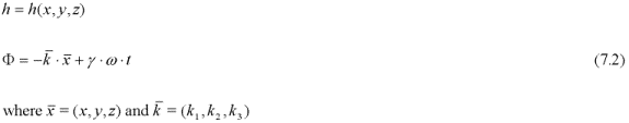
Applying (7.1):
We then get the transformed functions:
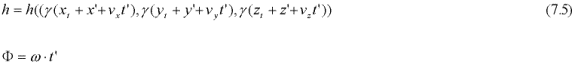
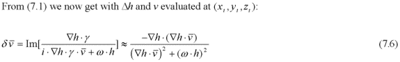
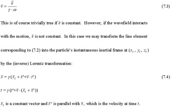
This holds for low velocities if h(...) is real valued. By Lorentz transforming (7.2) into the particle's instantaneous inertial rest frame we get (7.6) according to which the particle still might have a velocity relative to this inertial frame. In classical physics this velocity would be zero; instead there might be acceleration between the inertial frame and the particle frame. The difference here is due to the geodesic (7.1) that deals with velocity rather than acceleration. How this should be interpreted is not obvious. However, (7.6) might be seen as giving a velocity correction between consecutive discrete temporal frames. Perhaps the particle trajectory evolves according to (7.6) with time increments comparable to the period of the Compton frequency.
The geodesic may then be evaluated from the iteration:
Relation (7.6) gives a velocity change induced by the wave function h(...) that counteracts positive or negative motion in the direction of the gradient of the wave function striving to align a particle's trajectory perpendicular to the gradient vector. The geodesic trajectory depends on the locally changing wave function relative to the moving particle permitting both feedback interactions by self-interference and response to external influences.
8. The double slit interference experiment
Consider the double slit experiment in which a particle moves parallel to the x-axis toward a screen at x=0 with two narrow slits located at y=y0 and y=-y0. After passing the slits the particle strikes a second screen located at x = D, where an interference pattern develops even when particles arrive one at a time. According to the standard interpretation the particle somehow passes through both slits at the same time and "interferes with itself". David Bohm and others have shown that an interference pattern develops if the momentum relation (2.13) guides the particle, assuming that a wave function associated with the particle simultaneously passes through both slits. However, this does not explain how the particle is guided after passing through one of the slits and the physical mechanism at work. This problem is addressed here.
When the particle passes through one of the two slits, it might become slightly deflected and move in the y-direction as well as the x-direction. The matter-wave it generates interferes with the double slit geometry. Assume that the particle after passing the screen has the wave vector (kx , ky) and that its matter-wave interferes with the two slits generating a standing wave pattern :
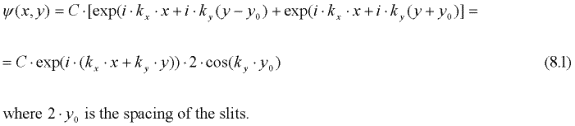
Defining the wave vector by:

Making the approximation:
So that:
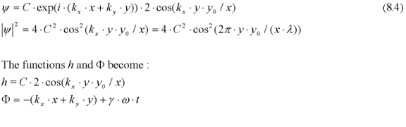
Relation (8.4) is identical to the classical expression for a light interference pattern. The resonance pattern is fixed in space and is determined by the geometry of the two slits. It expresses a potential that is activated by the particle's matter-wave, which resonates with varying amplitude in response to the particle's position and velocity. The wave function (8.1) represents the amplitude modulation of the Compton excitation if the particle is present at (x, y).
From (8.1) and the geodesic (7.1) we again get the trivial (7.3) assuming that the wave vector is constant. Following the procedure above Lorentz transforming (8.4) into the instantaneous rest frame we get:
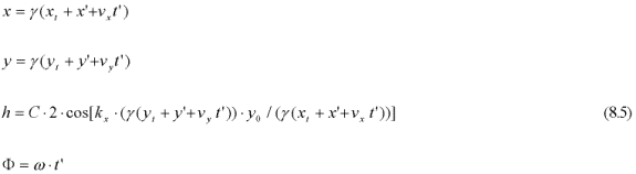
We have:
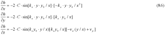
This holds true if kx is constant, i.e. if vx is constant. The geodesic (7.6) becomes:
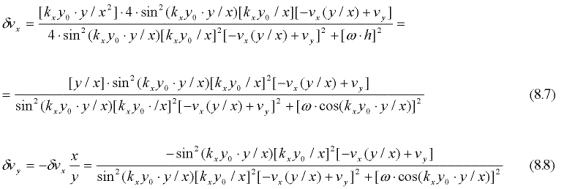
The velocity correction for vx is very much smaller than for vy if y<<x, which justifies the assumption that kx is constant. The particle's direction changes as long as vy/vx differs from y/x, i.e. as long as the particle does not move on a straight line from the origin at x=y=0. Since the particle passes through one of the two slits it does not come from the origin and its direction will change to align itself with one of the resonance ridges of the wave function. Between these ridges where the wave function is zero we have:
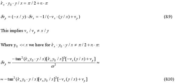
Thus, the particle avoids regions where the wave function (8.4) is close to zero. The direction changes rapidly close to the slits but slower with increasing distance, x, from the slits.
Figure 1

This explains the interference fringes around each (positive and negative) resonance crest of the wave function and provides a physical explanation to the double slit particle interference phenomenon. The particle interacts with its own matter-wave occupying regions where the matter-wave resonates with the geometry.Simulations of trajectories based on (8.7) and (8.8) using the approach of (7.7) show that vy/vx converges rapidly to y/x, which means that the particle after an initial adjustment travels in a straight line from the origin. The direction y/x changes when the initial velocities vy change as shown in Figure 1. The particles prefer certain directions that form the fringe pattern on the screen. This gives a physical explanation for the double slit experiment.
Self-interference might also explain the stable states for electrons in an atom. Resonance defines regions (corresponding to different energy states) that confine the electrons. Motion in the radial direction is counteracted by the geodesic (7.6). The trajectories line up perpendicular to the radial gradient resulting in circular orbits. These regions are created when the matter-wave resonates with the geometry and with externally imposed energy potentials, for example the electrostatic field. The self-interfering matter-wave automatically confines the electron. Stable states are sustained by feedback since the electron's motion defines the matter-wave, which in turn resonates with the motion. The electron moves on a geodesic, which explains why it does not radiate electromagnetic energy.
9. Deriving the Schrödinger equation from GR assuming oscillating spacetime metrics.
Consider the modulated Minkowski line element:

As before, setting the Ricci scalar corresponding to this line element equal to zero results in the linear wave equation (6.2) and justifies the use of the complex notations. I will assume that this temporal oscillation is associated with a particle, for example an electron, and that it is confined to a small spatial, moving, region.
Now assume that the wave function ψ is of the following form:
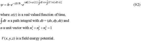
The line element then becomes:

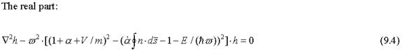
Carrying out the differentiations in (6.2) the "real" and "imaginary" parts satisfy:
We have:

The last term yields:

Also:
Combining the terms not depending on α in the real part we get the Schrödinger equation:

If also the remaining terms depending on α in the real part disappear we have:
The function α(t) is assumed only to differ from zero during transitions (jumps) between stable quantum energy states that are solutions to the Schrödinger equation, and to disappear between jumps. I will call α the "jump function".
Note that the direction of the vector n does not influence this derivation of the Schrödinger equation, which implies that the solutions only depend on the location and relativistic energy of the particle as given by it's Compton frequency. This suggests that the Schrödinger equation models resonance conditions of the spacetime metrics that only depend on the location and excitation (Compton) frequency of the particle.
The development above demonstrates that the Schrödinger equation can be obtained directly from the line element (9.1) by setting the linear part of the Ricci scalar, which contains second derivatives of the metric, equal to zero. Lorentz transformation retains the form of the wave equation (6.2) facilitating transformation between inertial frames. Although the form of the Schrödinger equation generally will change with a coordinate transformation, the line element representation (9.4) allows the corresponding wave equation to be derived in any coordinate system simply by setting the linear part of the Ricci scalar equal to zero.
The external field potential and the particle energy as given by the Compton frequency appear in the complex exponent modulating the metrics in (9.2) and the path integrals in the exponent model possible trajectories by the freely chosen unit vectors nk. We saw that the choice of the vectors nk does not influence the derivation of the Schrödinger equation.The function h, which is a solution to the Schrödinger equation, is the resonance amplitude generated by this superposition of motion in all possible directions. This wave function depends on the surrounding geometry and on the applied field potential V. When a particle moves, the wave field surrounding it creates resonance regions, which guide the particle via the generalized geodesic of section 7.If other particles also are present accompanied by their own wave fields, the resulting wave field is a superposition of all individual wave fields. However, since the particle's wave function is modulated by the Compton excitation, the wave functions from other sources, for example from different particles with different excitation frequencies (motions), will not interfere with a particle's motion.
With this interpretation the Schrödinger equation does not model the evolution of a dynamic process but models the passive response of spacetime to the presence of a particle at a certain location. Likewise, the time dependent Schrödinger equation models the passive response to the possibly changing Compton frequency of the particle. The resonating wave field determines the resulting trajectory subject to energy and momentum constraints.External influences, for example the presence of other particles with their associated wave fields, might influence the motion if the Compton excitation matches. In this way distant particles may interact via their wave functions. Furthermore, when the particle moves in a field potential its kinetic energy might change, which changes the resonance conditions of the metric field and as a result the trajectory might change via feedback action. This could influence the motion and confine the particle to resonating regions.
10. Quantum jumps.
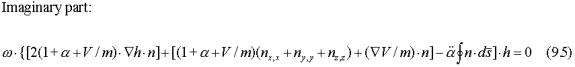
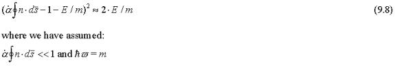
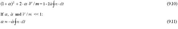
The jump function models the transition between discrete quantum states. Assume that initially the particle is in a stable state with some specific relativistic energy, which is reflected in its relativistic Compton frequency ωּγ. Suppose that a spatial excitation that matches the temporal frequency forms a standing particle-wave in the inertial frame of the particle. This standing wave is sustained by the oscillating metrics and I propose that a particle might be formed by a spatially confined resonance condition modulating both the temporal and spatial metrics. Now assume that a transition to a different quantum state given by the Schrödinger equation is accompanied by a sudden shift in the temporal frequency. This sudden shift in the Compton frequency also is accompanied by a change in the wave function h, which influences the particle's motion. However, initially this motion might not "track" the sudden shift. It is this transient mismatch that is modeled by the jump function α(t). Equation (9.11) implies that the jump function will converge to zero with time.However, we must then also require that the imaginary part of (9.5) disappears.
The second term in (9.5) contains spatial derivatives of the unity vector n and the assumption is made that this contribution is negligible. According to the EST theory the cosmological expansion progresses in temporal increments that induces oscillation in the scale, which is modeled by the line element (9.1). Due to the uncertainty relation the position of the particle is undetermined by a distance comparable to the Compton wavelength. This means that it is meaningless to consider any change in the direction of the particle in a time interval shorter than the Compton period. The vector n can therefore be thought of as a projection vector indicating the direction to where the particle will appear in the next step of the cosmological expansion process. I will assume that very short consecutive trajectory segments during which the vector n is constant model motion. Accordingly the trajectory of the particle is divided into small increments comparable to the Compton wavelength. During each of these very short intervals the direction of the vector n is fixed and its spatial derivative disappears.At each step k we may think of the vector n as pointing in the direction nk indicating where the particle will appear in the next step. With this assumption the continuous relation (9.5) is replaced by:
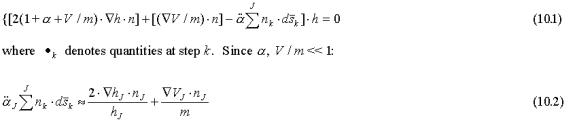
This relation models the jump process together with relation (9.11). The particle converges to regions where the product of the directional vector n and the gradient vector of the wave function is small, preferring regions where the wave function is close to either a maximum or a minimum. In the hydrogen atom the gradient of the radial wave function points in the same direction as the gradient of the electro-static potential V(r) and the trajectory approaches a circular orbit when α(t) approaches zero. In such a circular orbit the directional vector n is aligned perpendicular to the gradients of h and V so that the right hand side of (10.2) converges to zero with time. Even if the gradient of V differs from that of h, the ratio V/m is typically very small and the last term in (10.2) is negligible. On the other hand, the first term on the right hand side including the gradient of h could become very large close to zero crossings when wave function h is small. In a stable state the particle is therefore effectively confined within regions between zero crossings in agreement with the standard probability interpretation.
If the vector n points in the direction of the motion, the path integral corresponds to the total length of the jump trajectory. For example if we assume that the last term in (10.2) is absorbed in the second to last term and that the path length increases linearly with time:
11. The probability interpretation.
Born's interpretation that the squared magnitude of the wave function is a probability density is central to the standard interpretation of QM. However, the fact that Bohm's momentum relation is identical to the geodesic equation of GR suggests that the statistical interpretation of the wave function might be secondary. Bohm and Vigier [Bohm & Vigier, 1954], Belinfante [Belinfante, 1973] and Valentini [Valentini, 1991]] have demonstrated that the probability interpretation for the wave function is a direct consequence of the Schrödinger equation and Bohm's momentum relation (the geodesic) if one assumes that some additional excitation also is present. It is apparent from (2.14) that this is the case. An excitation in the form of induced high frequency acceleration is always present if the metrics oscillate.
Several authors have investigated the connection between the Schrödinger equation and stochastic processes that modulate particle motion subject to random disturbances. A recent example is the strictly mathematical treatment by Nelson [Nelson, 1982] who derives the Schrödinger equation from Brownian motion with three assumptions:
- Bohm's momentum relation applies.
- The energy is preserved.
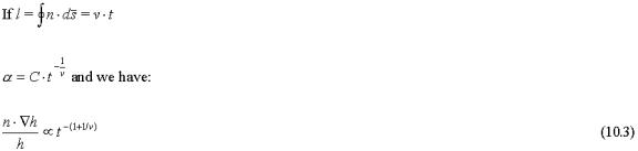
- A diffusion constant v is defined by:

The two first relations follow directly from GR for particles moving on the geodesics (2.13)) and the third corresponds to the uncertainty relation:

Thus, it appears that random motion, which is induced by the oscillating spacetime metrics and is constrained by GR and the uncertainty relation, characterizes the quantum world.
12. Summary
General Relativity and Quantum Mechanics might be closely related if the metrics of spacetime oscillate and a particle is accompanied, and possible sustained, by oscillation of the spacetime metrics at the Compton frequency.If this is the case the de Broglie's matter-wave arises as a relativistic effect when the particle moves. In addition, setting the linear part of the Ricci scalar equal to zero leads to Dirac type equations and the Schrödinger equation becomes part of a more general solution that also models quantum jumps.
In this interpretation the matter-wave is a purely relativistic effect created by moving oscillating metrics. The particle moves on the GR geodesic, which at low velocities is identical to the de Broglie/Bohm momentum relation.
Furthermore, the quantum mechanical wave functions are amplitude and phase modulations of high frequency oscillations in the spacetime metrics.If the wave functions are modulations of the spacetime metrics, they are not propagating waves in the ordinary sense but resonance conditions intimately depending on the local geometry and on the field potential. This explains how particles suddenly can jump between energy levels when shifts between different resonance modes occur. Spacetime oscillations could resonate with the motion of electrons in atoms. The electron automatically finds one of several possible regions and motions that sustain resonance.
This also could explain the enigmatic double slit experiment. The geometry of the two slits in the screen creates a spacetime resonance pattern that guides the particle by self-interference. Changing the geometry instantly changes the interference pattern. After passing through either one of the two slits in the screen the particle is guided by its own resonating matter-wave as determined by the double slit geometry.
The wave functions often are complex having both amplitude and phase. In the present interpretation this represents a phase shift of the modulated "carrier" oscillation. Therefore, the complex nature of the QM wave functions has clear physical meaning.
To summarize, if the metrics of spacetime oscillate, quantum mechanics may be derived directly from general relativity in a straightforward manner by setting the linear part of the Ricci scalar equal to zero. The quantum mechanical wave functions are then amplitude and phase modulations of a carrier oscillation at the Compton frequency associated with a particle and the de Broglie/Bohm pilot wave momentum relation is the geodesic of general relativity. This connection with general relativity may be used to derive a generalized momentum relation, which provides a clear physical explantion to the double slit experiment.
References:
Aspect A., 1986, Quantum Concepts in Space and Time, Oxford University Press. 1-15
Belinfante L.E., 1973, A survey of hidden variable theories, Oxford, Pergamon Press
Bell J. S.,1987, Speakable and unspeakable in quantum mechanics, Cambridge University Press, Cambridge.
Beller M., 1999, Quantum Dialogue, University and Chicago Press
Bohm D., 1952, A suggested interpretation of quantum theory in terms of "hidden" variables, I and II, Phys. Rev. 85, 166-193
Bohm D. and Vigier J.V., 1954, Model of the Causal Interpretation of Quantum Theory in terms of Fluid with Irregular Fluctuations, Phys. Rev. 96, 208-216
Bohm D., 1957, Causality and Chance in Natural Law, D. Van Nostrand, Princeton New Jersey
Bohm D., 1980, Wholeness and the Implicate Order, Routledge, London
Bohm D. and Hiley B.J., 1993, The Undivided Universe, Routledge, London and New York
Dirac, P. A. M., 1958, Quantum Mechanics, 4th ed. London, Oxford University Press.
Dürr J. S., Goldstein S. and Zanghi N., 1992, Quantum Equilibrium and the Origin of Absolute Uncertainty, J. Stat. Phys. 67, 843-907
Dürr J. S., Goldstein S. and Zanghi N., 1996, Bohmian Mechanics as the Foundation of Quantum Mechanics, in Bohmian Mechanics and Quantum Theory, An Appraisal, Kluwer Academic Publishers, Dordrecht
Holland P., 1993, The Quantum Theory of Motion. An Account of the de Broglie-Bohm Causal Interpretation of Quantum Mechanics. Cambridge University Press, New York, 1993.xx, 598 pp.
Home D., 1997, Conceptual Foundations of Quantum Physics, Plenum Press, New York and London
Kolesnik Y., 2000, Proceedings IAU 2000 (to appear)
Masreliez C.J., 1999, The Scale Expanding Cosmos Theory, Astroph. & Space Science, 266, Issue 3, p. 399-447
Nelson E., 1979, Connection between Brownian motion and quantum mechanics, Lecture notes in Physics, vol.100, Springer, Berlin
Penrose R., 1986, Quantum Concepts in Space and Time, Oxford University Press. 129-146
Popper K. R., 1982, Quantum Theory and the Schism in Physics, Hutchinson & Co. Ltd.
Valentini A., 1991, Phys. Lett. A, 111, 274-276