The Expanding Spacetime Theory

C. Johan Masreliez

1. Introduction.

The observed redshift of the light from distant galaxies suggests that the Universe expands. The assumption is usually made that this expansion results from spatial metrics that change with time. The idea of an expanding space naturally leads to the conclusion that the Universe originated in a spacetime singularity -- the Big Bang.

In this paper I show that there is a different mode of expansion for the Universe that does not imply a Big Bang type creation event. This new model, the Expanding Spacetime (EST) theory (formerly the Scale Expanding Cosmos (SEC) theory) agrees better with observations than the Standard Big Bang Model and resolves several cosmological enigmas.

2. A few remarks on the problem of modeling spacetime.

A pivotal development took place in cosmology when Einstein in 1917 (Einstein A., 1917) applied his General Relativity theory to modeling the Universe. His lead was soon followed by others, and with the discovery of the Hubble redshift, the expanding universe models suggested by Friedmann (Friedmann A., 1922) and Lemaître (Lemaître G., 1927) gained acceptance.

The basic idea of these expanding models is that the Universe evolves by changing the spatial metric relative to the temporal metric (expanding space while keeping the pace of time the same). This idea is philosophically attractive since it replaces Newton's absolute space with a space that expands, which eliminates the difficulty associated with an expansion into an absolute space that must have preceded the Big Bang.

However, taking a critical look at the Friedmann/Lemaître model and the considerations behind this particular choice of metrics, we find, as was carefully pointed out by Friedmann, that the temporal metric of the line element was chosen due to its mathematical simplicity rather than from physical or philosophical considerations. This simple form can always be obtained by suitable coordinate transformations of any general line element based on isotropy and homogeneity. However, there is nothing to support the contention that the choice of temporal metric in the Friedmann line element coincides with "natural time" defined by the pace of an atomic clock. Therefore, conclusions based on the Friedmann model regarding the nature of the cosmological expansion could be misleading.

Searching for an alternate to the expanding space model among an infinite number of possibilities requires reliance on observational data and on fundamental principles. I will show that a model exists based on two fundamental principles-equivalence between locations in spacetime and symmetry between space and time. This new model has the advantage of preserving the relationship between space and time so that the coordinate distance always coincides with the distance measured by timing a light beam. It agrees better with observations than the expanding space model and it provides simple explanations to several unresolved cosmological enigmas. In addition, this new model implies the existence of an inertial reference frame.

3. Definitions of a few terms and concepts.

The line element is of primary importance in cosmological models. In this paper spacetimes with line elements satisfying Einstein's General Relativity (GRT) relations identically are called "equivalent spacetimes" or simply "equivalent". In the same way different epochs with equivalent spacetimes are denoted "equivalent (epochs)". If there is equivalence and all laws of physics hold true then Einstein's "strong principle of equivalence" applies.

If all locations in space and time are equivalent then we have "global equivalence". This implies that metrics satisfy Einstein's GR equations identically everywhere in spacetime. They are equivalent for arbitrary translations in space and time.

If the Universe on the average is the same in all respects everywhere in space and time, the "perfect cosmological principle" applies. The perfect cosmological principle implies global equivalence. Global equivalence and the strong equivalence principle together imply the perfect cosmological principle.

If the metrics of space and time both are multiplied by the same positive factor, the "scale" of spacetime is said to be changed by a "scale factor". Spacetimes related by scale are called "scaled spacetimes".

"Absolute spacetime" denotes a spacetime with constant metrics for both space and time. If only the spatial metric is constant, the spacetime is called "space-absolute", and if only the time metric is constant, "time-absolute". The spacetime of Newton's universe is absolute. The Universe is usually assumed to be time-absolute but not space-absolute. The Expanding Spacetime is neither space- nor time-absolute.

A "Fundamental Location" is a location in space at rest relative to the average motion of particles in the Universe.

A "Fundamental Observer" is an observer stationary at a "Fundamental Location". "Natural Time" at any Fundamental Location is the time as measured by a stationary atomic clock.

4. Cosmologies based on the Perfect Cosmological Principle.

The perfect cosmological principle has in the past motivated the development of cosmological steady state theories, for example those by Bondi and Gold (Bondi and Gold, 1948), and by Hoyle (Hoyle, 1948). However, these theories assume that the cosmological expansion is time-absolute but not space-absolute. With this assumption the expansion opens up voids between galaxies, which are filled by the creation of new matter, for example the C-field cosmology proposed by Hoyle and Narlikar (Hoyle and Narlikar, 1962). The creation of matter and the Cosmic Microwave Background (CMB) are problematic for these theories. Superposed black body radiation at different redshifts does not preserve the black body spectrum in a spatially expanding universe.

The Expanding Spacetime (EST) theory of this paper, which also is based on the perfect cosmological principle, proposes that the Universe evolves by expanding the metrics of both space and time. This idea is motivated by the realization that the scale of material objects cannot be absolute in a completely relativistic universe. The scale of material objects ought to change with the scale of spacetime. The EST theory is a steady state theory, but no intergalactic voids are created since coordinate distances between fundamental observers remain the same measured with the expanding metrics. Thus, there is no need for continuous matter creation in the EST. I will also show that the EST is in thermal equilibrium, which explains the black body spectrum of the CMB radiation.

5. Spacetime scale equivalence.

Any attempt to model an expanding universe by Riemannian geometry leads to metrics that depend on time and therefore in general rule out equivalence between epochs. Furthermore, such a model based solely on spacetime geometry is like a map showing both the past and the future of the evolving universe but it does not explain the progression of time.

The EST evolves by changing the scale of spacetime rather than the geometry. This suggests that the line element evolves by a continuously changing scale, i.e. via a gauge transformation b(t):

However, the problem with gauge transformation is that GR no longer is covariant, which implies that different epochs are not equivalent. This suggests that GR might be generalized to include gauge transformation. Such modification of GR has been suggested by several authors in the past, for example Dirac (Dirac, P.A.M, 1973) who proposed that Einstein's General Relativity theory could be further generalized to include gauge transformation by using a geometry initially developed by Weyl (Weyl, H., 1921)). This idea is also followed up by Maeder (Maeder A., 1977) and Canuto et. al. (Canuto, V., et. al., 1977) in a series of papers.

However, if we restrict ourselves to GR we must consider discrete rather than continuous scale changes.

Spacetimes of different fixed scale are equivalent, which is realized by comparing the spacetime with metric g_ij, to the spacetime with the scaled metric b²·g_ij where b is some arbitrary constant. Einstein's General Relativity relations are given by:

As usual R_ijis the Ricci tensor, R the Ricci scalar, T_ij the energy-momentum tensor and k Einstein's constant. When applying these relations to the scaled metric we find that the constant b drops out from the left-hand side describing the geometry of spacetime. The left-hand side of these relations depends only on the metric g_ij. This implies that the right hand side, with the energy-momentum tensor T_ij, is identical for scaled spacetimes. Scaled spacetimes are therefore equivalent according to the definition above. But, are they strongly equivalent in the Einstein sense? We would expect this to be the case in a totally relativistic universe where there should be no preference between different scales of spacetime; all scales ought to be strongly equivalent.

Guendelman (Guendelman E.I., 1988) investigates scaled metrics and shows that under certain conditions a scaled metric b²g_ij can be formed from a base metric g_ij by a variable transformation. This automatically guarantees strong equivalence. Guendelman shows that one possible choice for such a base metric is:

Since variable transformation in GR implies that the strong equivalence principle holds, a (discrete) scale change must imply that the scale of matter depends on the scale of spacetime. If this were not the case, the energy-momentum tensors for spacetimes of different scales ought to differ. This equivalence of scaled spacetimes expresses of a fundamental symmetry property of the Universe.

6. The EST line element.

Although a scale expansion is conceptually simple, it is not self-evident how to model a cosmological scale expansion in General Relativity. Since relative coordinate distances in both space and time do not change, it may at first appear that the line element must be independent of time. However, a time independent line element ignores inertial effects.

An observer "traveling" with the expanding spacetime may be compared to a space traveler in an enclosed spaceship who tries to model the motion of the ship using only an on-board coordinate system. It is much easier to model the motions of the ship by using an external reference frame, for example an inertial frame coinciding with the on-board frame at some time t = 0.

I will use a similar approach and model the cosmological expansion relative to a fixed, non-expanding, coordinate system that coincides with the scale expanding system at t = 0.

Assume that the metric g_ij (t, x) has the form h(t)·g'_ij(t,x) where h and g'_ij are real valued functions, t, refers to the natural time coordinate and x to the three spatial coordinates. Temporal equivalence requires that two epochs corresponding to times t and t + t₀, where t₀ is some constant time interval, are equivalent. If b(t) is a real valued function of time it follows from the previous section that g_ij(t+t₀ ,x) is equivalent to g_ij(t,x) if:

This relation is satisfied if:

Temporal equivalence between all epochs requires that these relationships hold true for all times, t. This suggests a time dependency of the form:

C and T are constants. The scale factor b(t₀) is given by:

Since C is a scale constant it follows from the discussion above that we can set C = 1 without loss of generality. Also, since t₀ is arbitrary the time t can be put equal to zero at any epoch, for example the present epoch.

Furthermore, locations in space are equivalent for an arbitrary translation x₀ if a real valued function f(x) exists:

This suggests that the scale could change with spatial as well as with temporal location. One can easily show that such spatial scale changes imply gravitational gradients that would induce motion of matter in the Universe. However, the simplest case is when all the elements of g'_ij (x) are constants, for example if g'_ij (x) is the metric for a flat spacetime.

By this reasoning we arrive at the line element for the Expanding Spacetime:

This line element is the same as (5.3) found by Guendelman with a = 1 and C=T ^-2, which can be checked by making the variable transformation u =T x exp(t/T).Translation in time re-scales the EST line element, or interpreted differently, the cosmological expansion causes the progression of time. Since the EST line element is equivalent for all translations in spacetime, strong equivalence guarantees that the perfect cosmological principle holds. The EST Universe evolves by expanding the scale of everything while preserving all laws of physics as well as the spacetime energy density.

Since strong equivalence is obtained for a discrete but not for a continuous scale change, it appears that the progression of time in the EST must occur in discrete increments, or quanta, suggesting that the Universe expands by consecutive incremental scale changes. Thus, it appears that the expansion of the Universe might be generated by a series of consecutive "frames" like in a movie camera. What will happen in the next frame is governed by conditional probabilities based on previous frames. One might speculate that this mode of expansion could be the ultimate cause of quantum mechanics.

Expressed in spherical coordinates (6.7) becomes:

The flat space, without the scale factor e^2t/T will be denoted the "Coordinate Space". At time

t = 0 the Coordinate Space line element coincides with the Expanding Spacetime line element since the scale factor then equals one. However, the continually increasing scale factor causes several dynamic effects in the Expanding Spacetime. The quantity ds should be interpreted as proper time in an imaginary reference system with fixed scale. dt refers to natural time, which coincides with ds at t=0, dx=dy=dz=0.

There is of course the possibility that the spatial part of the line elements (6.7) and (6.8) is a curved three-dimensional space. However, at present there is no observational evidence for this. If the space is closed, which perhaps may be preferred from philosophical reasons, the radius could be considerably larger than the Hubble distance. An interesting argument in favor of flat spacetime is given by Guendelman (Guendelman E.I., 1988). Nature may have an affinity to flat spacetime since this is the choice of maximum symmetry. He argues as follows: "The reason background metrics that allow some conserved quantities for small perturbations around them are chosen by Nature may just be a phase-space reason, since, in that case, the small excitations can be degenerate (the degeneracy can be classified by the eigenvalues of the conserved quantities) and , therefore, we can have a high density of states around those states; then, the Fermi golden rule tells us that we have high transition probabilities if the conserved values have a continuous range of eigenvalues."

Since there is no absolute time, it is convenient always to use the present time as a reference. The line element (6.7) or (6.8) is given relative to the cosmological scale at the present epoch, which is normalized to one. Since the same line element applies relative to any epoch, there is a continually ongoing re-normalization process. This process is based on the fact that the line element with scale factor exp[(t+Δt)/T] is equivalent to the same line element with scale factor exp(t/T). Thus, the scale expansion could be modeled by considering a short time interval [t, t+Δt ] during which the line element (6.7) applies. At the end of this interval the line element is re-normalized by the substitution (t + Δt) => t and the process repeated for a new interval [t, t+Δt ] and so on. This substitution amounts to a discrete decrease in the pace of proper time ds=>ds exp(Δt /T). The factor exp(Δt /T) falls out restoring the EST line element. This permits the Universe to expand without changing the line element as applied to Einstein's equations. The spacetime geometry always remains the same and all epochs are equivalent. The Universe expands via discrete reductions in the pace of time while always keeping the geometry of spacetime the same. The spacetime geometry always complies with the GRT, but the progression of time is modeled by a stepwise, quantum expansion of the scale that is implemented via discrete, incremental, time translation. In this way GRT becomes covariant not only for continuous variable transformation but also for discrete scale expansion. This might be the much sought after connection between spacetime geometry and the progression of time. It permits cosmological evolution while preserving the perfect cosmological principle. The Universe is forever evolving yet always the same. It is conceivable that this scale expansion is not perfectly synchronized but varies slightly between sub-microscopic regions in space, creating a quantum mechanical spacetime "froth".

The scale expansion may be visualized by the following thought experiment. Assume that it would be possible to "freeze" the scale at a certain moment and observe the Universe from this vantage point "outside" spacetime. It would then appear that all distances were slowly increasing including the size of all objects and that the progression of time was slowing down as modeled by the EST line element (6.7).

The line element (6.8) is similar to the de Sitter line element (de Sitter, 1917):

Relation (6.8) models an expanding spacetime while (6.9) models an expanding space. Relation (6.8) applies to any location and any epoch of spacetime by setting r = t = 0 at any arbitrary origin. All epochs and spatial locations are equivalent. The distance, r, is the natural Coordinate Space distance from the selected origin and the time interval, t, is the natural time as measured by a stationary clock. This time scale is not arbitrary since t measures the aging process; for example the number of cycles counted out by an atomic clock.

The elapsed time, te, from t = -∞ to some prior epoch at time, t, as measured in "the present" time rate can be found by setting dr = dΩ = 0 and integrating:

a(t) is the scale of the Universe at time, t, relative to the present time where t = 0 and a = 1. We find that te = T at t = 0 showing that the age of the Universe as measured with the present time scale is finite and equal to T. Since the time can be put equal to zero at any epoch, this is also the age of the Universe relative to all observers regardless of the epoch.

The Hubble time, T, is therefore a universal constant that is the same for all epochs.

The time interval T has no relation to the aging process; it is just the time constant for the expansion. The changing time scale explains this somewhat puzzling statement. To see this let the Hubble time, which is the age of the Universe measured by the present time scale, be T seconds and the length of a second (at the present time) be unity. Since the metric of time expands, the length of the second at time (T+1), measured with the present metric, is approximately equal to ( 1+1/T). In "T-time", i.e. in the present metric, the "age" of the Universe at time (T+1) is equal to T+1. However, in the (T+1)-time metric the age of the Universe remains equal to T since T·(1 +1/T) = T+1. The time interval T can be viewed as an infinite sum of preceding time intervals (seconds) of decreasing duration's proportional to exp(t/T) as measured relative to the present time scale. The same holds true relative to all epochs.

The time, t, which is the natural time corresponding to the aging of matter, could be denoted the "aging time scale". It stretches infinitely back into the past. The pace of the aging time decreases with time. At present the aging clock progresses at a pace denoted the "present pace of time". Measured with an imaginary clock, which runs at a constant pace equal to the present pace, the "age" of the Universe is finite and equal to T. This time basis could be denoted the "present time scale". These two time scales are shown in Figure 1 assuming T = 10 billion years.

Differentiating (6.11) yields at t = 0:

This simple but illuminating relation tells us that the scale expansion is intimately related to the progression of time.

From (6.11) it also follows:

We get for the age, t_a, of an object:

This implies that the aging of stellar objects can be unlimited and explains why some stars in the Milky Way can be older than the Universe, i.e. how it is possible that t_a > T. For example, a 20 billion year old star was created at the epoch a = 0.14 assuming T = 10 billion years. The epoch a = 0.14 refers to a time where the scale of the Universe was 14% of the current scale. In the present time base this epoch lies 10·(1-0.14) = 8.6 billion years back in time. In the same way a 100 billion year "aged" object would only be 9.9995 billion years old in the present time scale (again assuming T = 10 billion years).

Light reaching us from the epoch a comes from the distance:

We have already seen that by making the transformation:

The line element (6.8) becomes:

This is a Robertson-Walker type line element. Although (6.8) and (6.17) are mathematically equivalent the temporal coordinate is not the same since (6.8) describes a cosmos without a beginning of time while (6.17) models a cosmos with "time" beginning at u = 0. The quantity u is not the aging time but a parameter proportional to the scale factor a (relation 6.16).

Formally treating u as a time parameter the redshift becomes:

The coordinate distance corresponding to this redshift is from (6.15):

This is the distance-redshift relation for the "Tired Light" model discussed by Geller and Peebles (Geller and Peebles, 1972) and LaViolette (LaViolette, 1986). I will return to this below.

The redshift is displayed in relation to the present and aging time scales in Figure 1.

Consider the transformation of (6.8) below, which first was introduced by Milne. (Milne, 1948):

The corresponding line element is:

In this expression r and t are functions of r' and t' given by (6.20). The r', t' spacetime is "radially" flat. It has several interesting properties.

For small t' and r' values we have from (6.20):

The Coordinate Space therefore locally coincides with the r', t' spacetime (except for the translation T).

Differentiating (6.20) results in the following expression for the velocity dr'/dt':

Noting from (6.20) that:

(6.23) becomes:

If the coordinate velocity dr/dt is equal to zero, (6.23) reduces to:

Because of the re-normalization process we have t = 0 and t' = T. Relation (6.26) is Hubble's Law with the Hubble constant 1/T.

The "expansion velocity" v = dr'/dt' creates a "Doppler type" redshift given by:

This agrees with relation (6.18) since r = - t for light.

According to (6.25) and (6.26) the observed velocity dr'/dt' is formed as the relativistic addition of the coordinate velocity dr/dt and the "expansion velocity" r'/t'.

Furthermore, according to (6.27) world lines in the Coordinate Space for which r is constant become straight lines through the origin in the r', t' spacetime as illustrated in Figure 2a and 2b. Due to the continuous re-normalization of the line element, an observer in the r', t' spacetime is always located at r' = 0, t' = T. Light cones backward in time from this location are straight lines. Figure 2b shows these light cones in relation to the world lines. When r approaches infinity, the world lines converge toward a straight line with slope equal to one. An infinite number of equidistant world lines are densely compacted close to this asymptotic world line. All these world lines have segments inside the light cone. This means that all locations in the Universe communicate and always have communicated. There is no particle horizon.

Although the Universe may have infinite extension, all locations are in continuous communication. This resolves the so-called Horizon Enigma.

Also, the Expanding Spacetime has no event horizon. All present events, regardless of their locations, will become visible by all observers at some time in the future. With respect to the particle- and the event horizons the Expanding Spacetime therefore behaves like a flat spacetime of infinite extension.

From (6.20) it also follows that:

Each epoch is therefore constrained to a certain hyperbolic surface in the r', t' spacetime. Of particular interest is the epoch a =1 which corresponds to the present time. The surface corresponding to this epoch is tangent to the r', t'-space at t' = T. The r'-space therefore locally coincides with the Coordinate Space for r<<T.

An observer, who assumes that the Universe is like the flat Coordinate Space with time progressing at an even rate will naturally make the mistake of believing that the extension of his locally flat space actually is identical to the r'-space. Redshifts caused by the expansion will then be interpreted as velocities in the Coordinate Space, i.e. it will seem like galaxies are moving apart when in fact these galaxies actually are at rest relative to the Coordinate Space.

The cosmos model expressed by the relations (6.20) is similar to the cosmos model suggested by Milne but with two fundamental differences. In the Milne model T is the time elapsed since the creation of the Universe. This parameter increases with the expansion of the Universe causing the Hubble constant to decrease with time. In the Expanding Spacetime model the parameter T is constant. The model is stationary since the observer will always be at r' = 0, t' = T. The Hubble constant is always the same, H =1/T.

A second difference is that the parameter r, which in the Milne model does not have any particular physical meaning, is the coordinate distance in the Expanding Spacetime model.

The Milne model was developed to describe the observed Universe, in particular the redshifts and the Hubble Law. It has been shown here that this model also describes the Universe as it will appear to an observer when both space and time expand simultaneously.

7. The Cosmic Energy Tensor.

When applying Einstein's General Relativity Theory to cosmology, the usual approach is to search for possible solutions to the Einstein relations based on some assumed energy-momentum tensor. It is generally believed that the only significant contribution to the energy-momentum tensor is the cosmological mass density plus radiation and that the energy-momentum tensor for vacuum is identically equal to zero. One well-known solution based on this assumption leads to the "Standard (Big Bang) Model" of Universe.

The assumption that the only contribution to the energy-momentum tensor is the cosmological mass distribution is questionable since it appears that the Universe contains more energy than what is contained in baryonic mass and radiation. This has motivated a so far futile search for the missing mass. However, there is another possibility - perhaps the assumption that the cosmic energy is dominated by mass is erroneous.

Einstein's General Relativity equations are usually stated in the form (5.2), which is interpreted as saying that the curving of spacetime (left hand side) is caused by the energy density (right hand side). However, these equations may also be put in the equivalent form:

This relation could be interpreted as saying that the energy distribution in the Universe is caused by spacetime curvature. The view that the geometry of spacetime defines the energy-momentum tensor is as valid as the view that the energy-momentum tensor decides the geometry of spacetime. Both views apply - the energy defines the spacetime geometry and vice versa.

Instead of postulating some energy-momentum tensor and then deriving the corresponding line element, I will take the opposite approach and assume that a certain spacetime curvature determines the energy-momentum tensor for vacuum. This curving of spacetime is generated by the scale expansion and the energy momentum tensor for vacuum is the tensor satisfying Einstein's General Relativity equations given the Expanding Spacetime line element (6.7). The energy-momentum tensor for vacuum therefore directly follows from the principle of equivalence.

Substituting the Expanding Spacetime metrics given by the line element (6.7) into Einstein's relations (5.2) we find that these relations are satisfied with the following energy momentum tensor T_ij setting c = 1:

The off-diagonal elements are all equal to zero.

This form of energy-momentum tensor is also considered by Kolb ( E.W. Kolb, 1989) in the context of the spatially expanding Universe where it models a forever coasting expansion at a constant rate.

The equivalent mass density corresponding to the energy density component T₀₀ equals the critical mass density. Therefore, there is no missing mass - spacetime itself contains energy equivalent to the critical mass density.

The tensor T_ij could be the fundamental energy-momentum tensor for the cosmos - the energy-momentum tensor of vacuum. I will call it the "Cosmic Energy Tensor". It is invariant for all fundamental observers regardless of their location or epoch.

The equivalent gravitating energy corresponding to the Cosmic Energy Tensor is zero since the sum of the diagonal elements is null (zero equivalent mass density). This suggests the possibility that, although the net energy content of vacuum is zero, the energy-momentum tensor of vacuum is not identically equal to zero. The principle of equivalence implies a Cosmic Energy Tensor with zero net gravitational energy consisting of components, which contribute equal amounts of positive and negative energy. The spatial expansion, which corresponds to the de Sitter line element (6.9), creates a Cosmological Constant (equal to 3/T²) with negative equivalent energy. This negative energy is in the Expanding Spacetime balanced by the temporal expansion, which has the effect of generating a cosmological pressure with positive energy density. Informally, the Cosmic Energy Tensor may be viewed as the sum of a Cosmological Constant corresponding to the spatial expansion and a Field Pressure due to the temporal expansion.

Thus, the equivalence between locations in spacetime implies that vacuum may contain energy that corresponds to the critical mass density. Therefore, spacetime itself, not matter or radiation, might contain the "missing mass" and is the primary fabric of the Universe.

8. The Ω - enigma

The circumstance that the cosmological baryonic mass density presently is less than one tenth of the critical density is surprising if the Standard Big Bang Model were valid. Dicke and Peebles, (Dicke and Peebles, 1979) noted that since the mass density now is so close to the critical mass density, the mass density in the early spatially expanding Universe must have been almost exactly equal to the critical density, i.e. omega must have been extremely close to one in the primordial Universe. This would be an almost impossible coincidence if the Universe were created in a (non-inflationary) Big Bang.

However, in the Expanding Spacetime the scale expansion is an "expansion without motion" which preserves distances between fundamental observers. This also implies that the mass density will remain constant during the expansion.

9. Spacetime geometry of the Expanding Spacetime.

Since the Coordinate Space is flat, the Expanding Spacetime is distortion free in the sense that it preserves spatial angles and angular directions for an object at a fixed location in the Coordinate Space. The expansion is conformal. Furthermore, since the cosmos expands by changing the scale of everything, it is clear that spatial angles and radial directions must be preserved during the expansion.

The Expanding Spacetime is also free of time dilation; i.e. a dynamic process would appear to evolve at the same rate as viewed by any observer in the cosmos. This follows directly from the line element (6.7), which preserves the relationship between space and time. Consider for example an observer at a coordinate location r_e sending a light beam to another observer at r_r. The observer at r_e measures the same photon rate using his local time base as the receiver does in the receiving time base at r_r. To the observer at r_r it appears that the signal is coming from a location r_e in a flat Coordinate Space where it is transmitted at the same rate as it is received. A distant observer of our solar system will therefore find the duration of the earth year to be the same as we do.

This property of the Expanding Spacetime also guarantees that a "light clock" consisting of two stationary, spatially displaced mirrors with a light beam going back and forth between them will measure out a time that agrees with the local atomic time at both mirror locations. Compare this with the situation when the spatial metric expands relative to time. In this case a light clock between fundamental observers will not agree with a stationary atomic clock. Since this would invalidate the foundation for Special Relativity it forces the assumption that there can be no local expansion of spatial metric in the Big Bang model.

Since the angular (or directional) geometry of the Expanding Spacetime is that of a flat space, the intensity of radiation from a source is proportional to 1/r² where r is the coordinate distance. Usually there are two dynamic effects of the cosmological expansion - redshift and time dilation. Since there is no time dilation in the Expanding Spacetime the only dynamic effect of the expansion is the redshift, which decreases the received radiation energy by a factor 1/(z+1).

It follows that the radiation intensity from a source with luminosity L is given by:

Using relation (6.19) we get:

10. Observational evidence for the Expanding Spacetime.

Sandage reviews three standard cosmological tests based on astronomical observations (Sandage, 1987):

1. Number count, N(m) or N(z), distribution.
2. Magnitude as a function of redshift - the Hubble diagram test.
3. Angular size - redshift test.

These tests are designed to test the validity of candidate cosmological models.

It has long been known that the Big Bang theory is failing tests b and c, (Sandage, 1987). Furthermore, recent observations (Metcalfe et a., 1995) show that it also fails the number count test.

However, the observational evidence refuting the Big Bang theory is largely ignored. Instead attempts are being made to save the theory by speculating that evolution over time is changing the number count, the luminosity, the size of radiating sources, etc.. In fact, the belief in the Big Bang theory is so unshakable that any deviations between this model's predictions and observations routinely are explained as being caused by evolutionary effects. Often no serious attempts are made to explain or justify these assumed evolutionary processes.

On the other hand it has been demonstrated convincingly by LaViolette (LaViolette, 1986) and others that the Tired Light redshift mechanism satisfies all cosmological tests without having to rely on evolution.

The simple angular size - redshift test is particularly decisive. An object with cross section d will be viewed at an angle given by:

Figure 3 is from a paper by Djorgovski and Spinrad (Djorgovski and Spinrad, 1981). The two dashed curves are the expected angular size-redshift relations for the Big Bang model with the deceleration parameter q and density ratio omega both equal to zero and one respectively. These predictions clearly deviate from the observations at large z values. The heavy solid line is relation (10.1). The agreement with observations for the Expanding Spacetime (Tired Light) model is striking. The angular size discrepancy is also dramatically confirmed by the recent Hubble Deep Field exposure. Distant galaxies appear to be much smaller than nearby galaxies using the standard Big Bang model distance estimates.

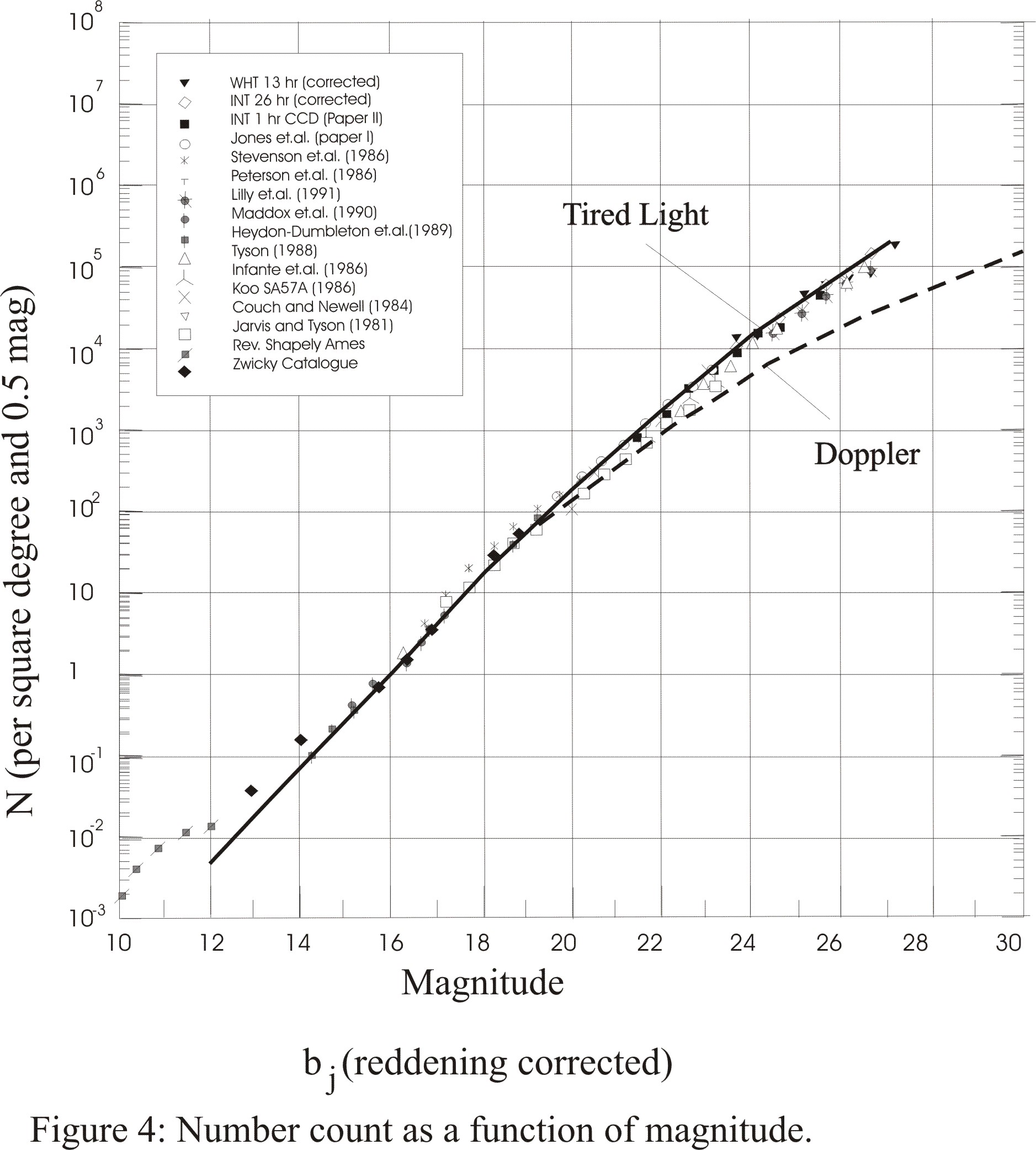
Metcalfe et. al. (Metcalfe N. et. al., 1995) summarizes the results from sixteen recent papers presenting observations of number count vs. magnitudes with magnitudes ranging from 14 to 27.5. Some of their results are presented in Figure 4, which is similar to Figure 10 in Metcalfe et. al.. The heavy line fits the tired-light redshift model to the data. Again, the agreement with the observations is excellent over the whole range, much better than attempts to fit various Big Bang models based on evolution.

The close agreement between the Tired Light model and the data of Figure 4 suggests that this data may be used to estimate the average galaxy luminosity and the galaxy number density. According to the Tired Light model the number of galaxies within a spherical volume increases with the redshift as:

N₀ is the number density. From (9.2) the magnitude, m, is given by:

Since the number count in the graph refers to 0.5 magnitude intervals and a one-degree spatial angle, the number count has been reduced by a factor 10^-5.

The good fit of figure 4 is obtained with C₁ = 24 and log(C₂) = 4.65. C₂ determines the relationship between magnitude and redshift, i.e. the curvature of the graph. C₁ represents a vertical translation.

The absolute magnitude M of a typical galaxy may be estimated from the relation:

r_mpcs is the equivalent distance in Mpcs:

With T = 10 billion light years = 3.07 thousand Mpcs we find from the data that M = -18.5. The absolute magnitude of the Sun is about +5 and its luminosity:

Based on this the estimated average galaxy luminosity becomes:

This implies an average inter-galaxy distance of about 4.3 Mpcs. This estimate has the usual uncertainty due to the uncertain Hubble constant. Both the estimated mean galaxy luminosity and the number density agree well with previously available estimates.

11. The Cosmic Microwave Background.

The Cosmic Microwave Background (CMB) is generally believed to be remnant radiation from the Big Bang creation. However, I will argue that the EST is in thermal equilibrium and that the CMB may naturally result from thermalization of existing electromagnetic radiation.

Since the EST expansion preserves the energy momentum tensor and the strong principle of equivalence applies between epochs, the electromagnetic radiation energy density in the Universe must remain constant during the expansion. This implies thermal equilibrium. In a recent paper Assis and Neves (Assis and Neves, 1995) point out that the Tired Light model predicted the correct temperature of the CMB in a Universe with thermal equilibrium long before measurements were available. A temperature of 3.2K for the Universe was predicted as early as 1926 by Eddington (Eddington, 1926) based on stellar radiation assuming a static universe in thermal equilibrium. Independently Regener (Regener, 1933) estimated a temperature of 2.8K using Stephan-Bolzmann's law assuming that the energy source was cosmic radiation. This was confirmed by Nernst (Nernst, 1937). The close agreement between these early estimates and the CMB temperature of 2.73K is noteworthy. Thus, it has long been known that the CMB is a natural phenomenon to be expected for a Universe in thermal equilibrium like the Expanding Spacetime.

To further support this claim I will show that the Planck black body spectrum is preserved in the EST. Since it seems to be difficult to analyze a situation where both the spatial and the temporal metrics expand simultaneously, it is easier to consider a line element with constant time metric like the line element (6.20). The corresponding, transformed, spacetime may then be analyzed assuming that standard physics apply.

An observer in the bounded spacetime of line element (6.20) will experience the Universe as a stationary spherical cavity containing innumerable radiation sources (galaxies). The vast majority of these galaxies are located at, or close to, the horizon where the space is infinitely compressed by the expansion. Furthermore, since the coordinate space is assumed to be unbounded, almost all of these sources are located at huge distances where the radiation from them, as seen by an observer, is intercepted by intergalactic and galactic matter. The radiation from these innumerable sources will therefore reach an observer from enormous distances. The angular intensity variation should be minimal if the Cosmological Principle applies. This has been confirmed by the recent COBE satellite measurements as reported by Smoot et. al. (Smoot et. al., 1991 and 1992).

The spacetime of line element (6.20) does not generate a time dilation type redshift since it is radially flat. Instead the expanding volume generates the redshift. The volume element corresponding to the line element (6.20) is given by:

This may be compared with a volume element in the coordinate space:

Furthermore from (6.19):

From (11.1), (11.2), (11.3) and (11.4) it follows:

Since the line element of (6.20) coincides with that of the flat coordinate space at z = 0 and since the CMB energy density is the same everywhere in the Coordinate Space, the CMB energy density at a distance corresponding to a redshift z will in the spacetime of line element (6.20) appear to be increased by a factor (z+1)⁴.

Assume that the a volume element at a distance corresponding to redshift z relative to an observer in the transformed space of (6.20) radiates with a black body spectrum given by:

where l is the wavelength, h is Planck's constant, k is Boltzmann's constant, and T⁰ is the black body temperature.

According to the development above the spectrum of the received light at z = 0 is attenuated by a factor 1/(z+1)⁴:

Letting λ' = (z+1)·λ we find that the received light also has a black body spectrum but with a reduced temperature T' = T⁰ /(z+1):

This shows that the black body character of the CMB spectrum is preserved. Black body radiation generated at some temperature and distance will be received as black body radiation at the same temperature. Stated differently, black body radiation emitted at the temperature T⁰ at a redshift z will relative to an observer in the spacetime of (6.20) seem to have been emitted at the elevated temperature T⁰·(z+1). However, the temperature of this radiation will be reduced by the factor (z+1) before reaching the observer. Therefore, the black body radiation is the same at the emitter and the receiver. Like in a flat spacetime, black body radiation is in equilibrium in the EST. This may be compared to the spatially expanding model, where the volume element is proportional to (z+1)^-3. Since the emitted CMB energy density is proportional to (z+1)⁴ the black body radiation spectrum can only be preserved if all CMB radiation actually were emitted at a temperature T⁰·(z+1). In the EST model the expanding temporal metric adds the missing fourth dimension.

The Expanding Spacetime has the interesting property not shared with the spatially expanding universe, that the black body radiation is in equilibrium. In this respect it behaves like a classic stationary cavity. Any region of the Universe radiating with a certain black body spectrum will be in equilibrium with other regions radiating with the same spectrum. The only thing needed to generate a black body spectrum in the Expanding Spacetime is a source for the energy. If this energy is available, thermalization processes will automatically generate the black body spectrum given enough time, since this spectrum is the spectrum of highest probability (entropy).

There is another way to see why the EST must be in thermal equilibrium - there must be some temperature at which the energy lost by redshifting equals the energy added by radiating sources. If the average number density of these sources is N, their average luminosity L, and the equilibrium energy density E, we have due to the Tired Light redshift effect:

With the estimates (10.9) and (10.10) the energy estimated from (11.9) is about two orders of magnitude too small. However, many galaxies radiate over ninety percent of their energy in the infrared and since the equilibrium energy, E, includes all electromagnetic energy from the radio frequencies to gamma rays, relation (11.9) could still hold.

On the other hand, in a spatially expanding cosmos like the Big Bang universe, thermalization will generally not result in a black body spectrum since superposition of black body radiation at different redshifts destroys the black body character of the spectrum. Therefore, all of the CMB must in this case come from the "primordial fireball" of the Big Bang. There can be very little thermalizing processes in the spatially expanding universe if the CMB black body spectrum is to be preserved.

Thus, the CMB is a natural phenomenon to be expected in the Expanding Spacetime while very special conditions must exist to explain the very uniform CMB temperature in a spatially expanding universe.

12. Geodesics in the Expanding Spacetime.

The General Relativity geodesic relations are given by:

All other Christoffel symbols are zero.

The geodesic equations are:

Integrating with K as an integration constant:

I will call this property of the EST "cosmic drag".

The length of a geodesic, Lr, for a particle with non-zero rest mass is finite and may be obtained by integrating (12.12) from zero to infinity:

This might be compared with (6.28). Setting:

The redshift when the particle finally has come to rest is the same as the initial redshift. In the Appendix 2 I show that the redshift remains the same at all times giving the impression that the particle moves away at a constant speed rather than being slowed by cosmic drag.

Thus, the relative velocities of freely moving particles with non-zero rest mass will decrease with time in the EST. Since these geodesics have finite lengths, all particles will eventually come to rest relative to each other, discounting the effect of the Field Pressure. Therefore, all inertial coordinate systems will converge and will (except for coordinate rotations) merge into one single coordinate system in the infinitely remote future. The retardation of inertial coordinate systems also implies an asymmetry in the equations of motion, which defines the direction of time.

For velocities much lower than the speed of light this reduces to:

The energy of a particle with mass m and rest mass m₀ is given by:

From (12.10) and (12.11):

This is the Tired Light redshift mechanism.

13. The question of an inertial reference frame.

The cause of inertia has been an enigma since the time of Newton. Since inertia undoubtedly exists, a cosmological model without some kind of inertial reference frame is unthinkable. All models of the universe assume that a rest frame exists and the Expanding Spacetime theory does not differ in this respect. However, the advantage with the Expanding Spacetime theory is that the cosmological scale expansion defines, or generates, a reference frame. Thus, the theory implies the existence of a cosmic reference frame.

The mechanism that generates the reference frame is the cosmic drag, which causes the relative velocities between galaxies and relative angular momenta to decrease with time. This explains why the relative velocities generally are much lower than the speed of light. Since galaxies on the average are at rest relative to each other, they define a rest frame much like in Mach's principle. Furthermore, since the cosmic drag also applies to angular rotation, a rest frame for rotational motions is also defined by the scale expansion. Unlike Newton's absolute rest frame that was assumed to exist in the absence of matter, or the expanding universe model where stable small relative velocities are postulated but not explained, there is a feedback mechanism in the Expanding Spacetime that guarantees that relative translational and angular velocities are small. These small velocities serve to define an inertial reference frame which no longer is absolute but which depends on the motion of matter in the Universe.

The reference frame is self-consistent. It serves as a reference for the scale expansion, which in turn defines the reference frame.

14. Spiral galaxy formation.

The cosmic drag effect may also explain how spiral galaxies are formed and how these thin rotating discs of billions of stars can remain stable over time. The stability of spiral galaxies cannot be explained by known physics without assuming some stabilizing agent, for example an invisible galactic halo (Ostriker and Peebles, 1973).

In the absence of any disturbance gravity, the equations of motion for individual stars of unit mass in a thin disc, given in an inertial frame with its origin at the galaxy center, can be written in cylindrical coordinates as (Chandrasekhar, 1960):

Since to objective of this brief analysis is to gain a qualitative understanding of the effect of the gravitational drag, the gravitational potential is for simplicity assumed to be a function solely of the radial distance r. In a more realistic model the angular component of gravitation will be important, in particular for a galaxy with a significant portion of its mass in the galaxy arms. The assumption is also made that the gravitational potential does not change with time although this could be of some significance due to accretion.

Relation (12.4) may be re-written as a function of time using (12.16) assuming that all velocities are much lower than the speed of light. We get after adding the gravitational acceleration:

G is the gravitation constant, M(r) the equivalent gravitating mass at radial distance r, and J is the initial angular momentum per unit mass. According to (12.16) for small velocities:

Relation (14.2) differs from the standard relation by the cosmic drag term -(dr/dt)/T and by the exponentially decaying angular momentum, which causes moving particles to spiral toward the gravitational center. Although the cosmic drag term is quite small it will efficiently dampen radial oscillations. The term within the bracket controls the shape of the spiral. If this term were equal to zero the solution of (14.2) would satisfy:

In a steady state situation the mass flow must be the same at all radial distances otherwise there would be a mass accumulation or depletion somewhere in the galaxy disc. This suggests that the gravitating mass may increase linearly with distance:

From (14.3) the velocity v becomes:

The velocity curve is flat.

The angle of rotation as a function of time is found by integrating (14.3) using (14.4):

Consider a spiral galaxy with arms reaching out past the distance r₀ and an observer located at an arm at this distance, moving together with the arm with the constant velocity v. Mass particles in the arm are accelerated radially and flow past the observer along geodesics toward to galaxy center. Since the mass flow in the arm is essentially laminar, and because particles move on geodesics, there are no shear forces. Matter flows along a galaxy arm toward the galaxy center like inside an imaginary tube.

The angular motion of a particle relative to our observer is:

The trajectory of particles relative to the observer, which may be found from (14.4) and (14.9), determines the shape of the galaxy arm.

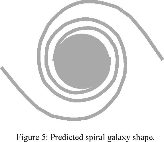
Using the Milky Way as an example, at r₀ = 100 kpcs the time corresponding to one full revolution of a spiral arm is approximately 7 billion years. During this time a particle's (stars) distance to the center has decreased from 100 to 50 kpcs. The observer at 100kpcs has completed 2.2 revolutions around the galaxy center and the star 3.2 revolutions. The corresponding shape of the galaxy arms is shown in Figure 5. A spiral galaxy usually also has a large fraction of its mass concentration at its center. This will modify both the shapes of the spiral arms and of the velocity curve. The shapes of the arms will also be modified by the angular component of the gravitational field when a significant portion of the mass is in the galaxy arms.

This discussion suggests that the spiral shape and stability of spiral galaxies may be explained by the cosmic drag effect, a conjecture that should be confirmed by further analysis supported by computer simulations.

15. Observational evidence for the cosmic drag effect-Pulsars.

Since the cosmic drag effect generally is quite small it is difficult to detect and measure it directly. However, the periods of signals received from rotating neutron stars, pulsars, are extremely stable and have been measured very accurately. The period increases slowly with time for most pulsars. This means that the rotating neutron star is losing angular momentum. If this loss of angular momentum is due to cosmic drag, we would expect that the spin-down will satisfy:

P is the period between pulses. Table 1 below shows the measured periods and their rate of change for 25 pulsars. The third column is the ratio between the period and its time derivative, which should equal the Hubble time if the spin down solely is caused by cosmic drag.

B is the estimated magnetic field strength in Gauss. The data was obtained from the papers by Danner, Kulkarni and Thorsett (Danner, Kulkarni and Thorsett, 1994), Burderi, King and Wynn

(Burderi, King and Wynn, 1995) ,van den Heuvel ( van den Heuvel, 1995) and Camillo et.al. (Camillo, Nice, Shrauner and Taylor, 1996). The last sixteen entries are members of binary systems. The parameter "e" is the eccentricity of the binary orbit. There is some uncertainty in the data since three sources reports the period derivative for the pulsar J0437-4715 as being 0.24, 1.2 and 0.4 · 10^-19 s/s respectively. Also, a recent paper by Nice and Taylor (Nice, D. J.and Taylor, J. H., 1995) estimates the spin-down time constants for the pulsars J2019+2425 and J2322+2057 at 5.6 and 4.9 times 10¹⁷ seconds respectively.

The striking feature of this table is that the spin-down time constants for many of the pulsars agree. It is very unlikely that this should be the case unless the spin-down is caused by some common effect. The observed spin-down time-constants also agree with a Hubble time in the order of 10-20 billion years except for a few of the pulsars. This lends support to the proposition that the slowing pulse rates are caused by cosmic drag. The spin-up of one of the pulsars could result from accretion of a nearby evaporating star.

In the E.P.J. van den Heuvel paper (1995) the author observes that the magnetic field strength seems to bottom out around 10⁸ Gauss. At this field strength the Alfvén radius is in the order of 10-20 kilometers, which is similar to the typical radius of a pulsar. Van den Heuvel proposes that at higher field strength a pulsar will accrete matter primarily at the magnetic poles with field polarization opposite to that of the pole. This accretion process will reduce the magnetic field strength until the Alfvén radius equals the radius of the neutron star. Any additional accretion after this point will accumulate randomly all over the surface and not reduce the field strength further. This suggests that a pulsar with very small accretion rate at the end of its accretion phase have a magnetic field strength in the order of 10⁸ Gauss.

The spin-down time constant is nearly the same for the all pulsars in the table with low field strength (and presumably low accretion). The average spin-down time constant for fifteen pulsars in the table with low field strength is 13 billion years, all values falling in the interval 3 - 25 billion years. Part of this variation is undoubtedly due to measurement uncertainties.

It is difficult to explain the observed spin-down rates by known physics. Consider a pulsar with a period of five milliseconds, with mass comparable to that of the Sun, and with ten kilometers radius. If such a pulsar were to be slowed down by friction only, the heat generated would be of the same order as the energy radiated by the Sun. Frictional forces can therefore not explain the spin-down. Furthermore, the deviation from rotational symmetry should be negligible due to the enormous force of gravitation at the surface. Therefore, insignificant energy is lost due to gravitational wave radiation. Also, tidal effects are insignificant for such a compact object and magnetic dipole braking is negligible with a magnetic field strength in the order of 10⁸ Gauss. Cosmic drag is the only conceivable explanation.

Cosmic drag could also help explain short orbital periods (in the order of a few days) for some binary star systems. Since tidal forces prevent stars from forming at these close distances, they must have formed separately at much larger distances. The cosmic drag will steadily diminish the inter-stellar distance over billions of years. The distance between binaries decreases with a time constant of half the Hubble time and the orbital period with a time constant equal to one third of the Hubble time. An initial orbit of 1000 days is reduced to 2.5 days in two Hubble times (about 30 billion years). Binaries with orbital periods in the order of days should therefore be very old. There is also a correlation between the eccentricity of binary orbits and the period of the orbit. The shorter the period is, the smaller is the eccentricity. This confirms the proposition that the orbital period decreases with time together with the eccentricity due to cosmic drag.

The agreement between spin-down rates for many pulsars and the difficulty in explaining these spin-downs strongly suggests that they may be a cosmological rather than a local effect. The confirmation of this conjecture would be a very significant finding. For example, if we could show that the spin-down time constant is the same for all non-accreting pulsars with low magnetic fields it would provide irrefutable evidence that the spin-down is due to a cosmological effect common to all pulsars.

The variability between estimates in the table is partly due to observational uncertainties and partly due to the particular data processing approach selected by the author. Using exactly the same data processing scheme should reduce the second source of variation and help confirm that the spin-down rates are the same for all pulsars. Obviously, this would be a very worthwhile project.

16. Astrometric evidence of the EST theory in the solar system.

The EST theory predicts secular accelerations of the orbiting bodies in the Solar system according to relation

where is the secular acceleration of a planet not taken into account in the adopted gravitational theory of the planetary motions, n is the mean motion of a planet and T is the Hubble time. The observations of planets provide corrections to their mean longitudes along with the respective secular variations in the form

(16.2)

The parameter t is the time in centuries. By differentiating (16.2) corrections to the theoretical mean motion of a planet Δn and its secular acceleration are defined respectively as , . The latter is the principal parameter to be discussed below. The estimates of the predicted semi-accelerations of the innermost planets (in arcsec/cy²) are presented in Table 2.

Table 2. Semi-accelerations of the innermost planets predicted by the EST theory

T ( billions of years )	Mercury	Venus	Earth
10	8.08	3.16	1.94
11	7.34	2.87	1.77
12	6.73	2.63	1.62
13	6.21	2.43	1.50
14	5.77	2.26	1.39
15	5.38	2.11	1.30
16	5.04	1.97	1.21

16.1 Optical observations of the planets

In order to understand the techniques and methods involved in confirming the minute accelerations predicted by the EST theory, let us consider the present status of optical planetary observations. The Sun, Moon and planets are observed differentially with respect to stars so that their observed positions are obtained in the system of a reference stellar catalogue. The principal axes and planes of this system are defined by a list of equatorial coordinates and proper motions of some subset of stars. The zero points of this set of coordinates are considered as equinox and equator of this stellar fundamental catalogue given at some standard epoch. In other words the "stellar equinox and equator" are conventional mathematical conceptions adopted by the astrometry community. In the ideal case these zero points should be in coincidence with the intersection of ecliptic and equator at some standard epoch defined by the actual motion the Earth around the Sun and rotation around its axis, i.e. the actual dynamical equinox "of epoch". Due to luni-solar precession, planetary precession and nutation the equinox and equator plane are continuously changing their positions in space so that at a certain moment of time we deal with the equinox and equator "of date".

Observations of planets are tied to reference stars and the positions of stars are calculated from their positions and proper motions of "standard epoch" by use of the adopted precession constant defined by the relation between the "stellar" equinox and equator "of date". By this procedure we obtain the observed positions of a planet in the stellar reference system. The observational data are published in the form of so-called "observed apparent places" (O) of a planet referred to a certain stellar system (FK3, or FK4, or FK5, or N30, or GC, etc) at the observed moment of Universal time (UT). This moment is either calculated from the observed right ascension as the sidereal time of the planet's transit and then converted into UT (that was traditional practice before atomic time became available) or recorded by an independent clock tied to Universal Coordinated Time (UTC), which represent one form of atomic time.

These positions are compared with the respective positions of the planet derived mathematically from a planetary theory, giving the "calculated theoretical apparent places" (C) at the time scale of this theory, i.e. Ephemeris Time (ET). The computed positions of planets are calculated at the time of observation given in UT by use of the difference ΔT=ET-UT, see below. Any planetary theory represent our actual knowledge of the planetary motions in the Solar system and gives as a result predicted positions of a planet for any moment of ET. By this it provides positions and orientations of the principal planes and points of planetary orbits thus defining the theoretical "dynamical equinox and ecliptic" or "dynamical reference system". The modern numerical ephemerides give planetary positions in the reference frame of a standard epoch so that to compare these with observed positions we use the precession transformation from a standard epoch to the epoch of date. Since the same precession constant is used for calculation of the apparent "stellar" and "theoretical" positions, which are compared, the error of this constant is subtracted and does not affect the results.

The results of the comparison are residuals (O-C), as usual in right ascension and declination. First of all, they give us information of the mutual displacement of the "stellar" and "dynamical" reference systems. Numerical characteristics of this displacement are so called "equinox correction" ΔA and "equator correction" ΔD. They have the sense of the angles by which the stellar system should be rotated to be coincident with the dynamical system. The secular trends in the equinox or (and) equator corrections are interpreted as the mutual residual rotation of the stellar and dynamical systems. In the scientific literature it is named as a "non-precessional" or "fictitious" equinox motion. In principle, the origin of rotation may be found either in the stellar system or in the dynamical system but the methodology of fundamental astrometry is based on the assumption that the dynamical reference frame is basic, unmovable and quasi inertial. Thus, any shift or rotation between the stellar system and dynamical system is assumed to be exclusively due to the stellar system.

On the other hand, a set of residuals (O-C) also gives information about imperfection of a planetary theory, i.e. in the simplest case, corrections to Keplerian elements of a theory are derived.

For analytical estimation of the orientation of the stellar reference frame and corrections to elements of Earth's orbit, the conventional conditional equations suggested by S. Newcomb apply for the Sun:

where ΔA and ΔD are corrections to the equinox and equator of a reference catalogue, ΔL_o is the correction to the origin of Sun's mean longitude, Δε is the correction to the obliquity of the ecliptic, Δh and Δk are related to corrections to the eccentricity of the Earth's orbit e_o and the longitude of perihelion π _o

For the planets the conditional equations are more complex. When long time spans are available for analysis, the terms in (16.2) with t and t² are added to derive secular variations of the equinox correction and correction to the mean longitudes of the Sun and planets. It is important to mention that due to the almost constant coefficients in some of the relations the estimated unknowns and their variations may be separated with a limited reliability. So, in the case of the Sun, since the coefficient at ΔL in right ascension is almost constant the secular variations of the equinox correction and the mean longitude cannot be effectively separated. However, this correction may in principle be derived from the declination residuals. In the case of Mercury and Venus the question is more complicated in view of correlation between elements of the Sun and planets but the tendency remains the same.

It follows from the above that the secular variations of residuals might be caused by the three principal factors:

1. residual rotation of a stellar system with respect to dynamical system;
2. secular errors of the Keplerian elements in the ephemeris of comparison;
3. errors in the adopted difference of Ephemeris Time and Universal Time.

16.2 Residual rotation of the system of the fundamental catalogues

Newcomb determined orientation of the first fundamental catalogue, FC, on the basis of observations of the Sun from 1756 to 1869. This equinox denoted as N₁ has afterwards been revised many times by incorporating different series of observations in the form of corrections ΔN₁. These numerous determinations of the equinox corrections have shown a negative linear drift from analysis of the 19^th century observations, the absence of a drift at the beginning of the 20^th century and subsequently an indication of a positive drift from observations in the middle of this century. However, the net secular drift of the equinox was found to be negligible. As a result, no correction was applied to the FK3 positions when the FK4 was introduced in 1964. But during the work with the construction of the next fundamental catalogue, FK5, evidence of a positive equinox drift of FK4 derived from many modern observations became so clear that Fricke (1982) derived his estimate of equinox drift 1.27"/cy. To construct the proper motion of the FK5 system, proper motions of FK4 were revised by corrections including a new precession constant and the secular drift of the equinox 1.27"/cy.

It was believed that after such a revision the FK5 would not show any discrepancy with the dynamical system. Ironically almost all planetary observations reduced in the FK5 reference frame have shown absolutely the opposite result. A nearly 1"/cy negative correction of the stellar equinox has been reported by different authors from analysis of more or less extended series of modern observations. Yao and Smith (Yao&Smith,1988) estimated a drift in the range -0.88"/cy to -1.18"/cy, (Kolesnik 1995, 1996) a drift from -0.92"/cy to -1.29"/cy, Poppe et. al. 1998) from -0.91"/cy to -1.03"/cy. The question is still unresolved. Where lies the origin of discordance? Are the proper motions of the FK5 infected by errors or are there discordance's between observations of the solar system bodies with respect to the FK5 stars? The latter case is usually regarded to be the least realistic since, as mentioned above, the dynamical reference system always has been considered errorless.

Now, an independent method to check the FK5's proper motions is appearing. The HIPPARCOS catalogue, in which all FK5 stars are included, is linked to the extra-galactic reference frame, and by this it is considered to be free from residual rotation. Comparison of the proper motions of these two catalogues has shown the absence of significant rotation at the level of 1"/ cy. In the equatorial zone we estimate it to be 0.1"/cy in the sense FK5-HIPPARCOS. This seems strange in view of the uncertainty in determination of the FK5 equinox. Moreover, in the study of the FK4 distant stars (Fricke 1967), the determination of secular variation of ΔA linearly depended on the derived correction to the general precession in right ascension ( -λ). The most recent revision of the IAU 1976 precession constant is -0.32"±0.13"/cy, which was obtained independently using lunar laser ranging and an interferometric technique by Herring at al. (1991). This means that if the 1.27"/cy equinox correction is absolutely correct, the proper motion of the FK5 system must have an additional rotation of about -0.30"/cy whereas as we observe only -0.1"/cy. The discordance is rather large compared to the reported 0.1 mas agreement between the HIPPARCOS extra-galactic frame and the FK5 stellar catalog.

This simple reasoning raise some doubts for a commonly spread opinion that extra-galactic reference frame is absolutely inertial and that it agrees with previous conceptions of the stellar kinematics and the adopted postulates of the planetary dynamics and the Earth's rotation. Anyway, comparison of the FK5 with HIPPARCOS indicates that the proper motions of the FK5 are not infected by large errors. However, rotation between stellar and dynamical reference frames is an empirical fact. This provides convincing evidence that the origin of the secular discordance in the planetary observations is to be explained by the two latter of the above stated factors, i.e. errors in the computed orbit (ephemeris) and/or error in the relation between UT and ET.

One study preceding the adoption of Fricke's secular equinox motion should be mentioned here. This is Blackwell's paper (Blackwell 1977) who analyzed position and motion of the equinox during past 250 years (from 1755 to 1971) and concluded that the equinox has a secular acceleration of about 1.3"/cy² relative to a stellar reference system rather than a linear drift. He presented numeric estimation of the secular variation of correction to Newcomb's equinox by the expression:

ΔN = -0".55+0".1(t-19.00)+0".66(t-19.00)² .....................(16.4)

Although he did not offer any explanation for the physical cause of such variation, this empirical relation agrees with a numerous separate determinations of the equinox and with their straight-line solutions for its drift. The latter ones were fitted to the limited spans of the parabola at the respective epochs, see the Figure 1 of his paper.

16.3 Deceleration of the Earth's rotation and the relation between ET and UT.

Secular variation of the Earth's rotation introduce cumulative discrepancy between Universal Time and a time-like argument of planetary theories that is manifested in secular variation of corrections to the mean longitudes of planets. After the study by Spencer Jones (1939) the effect of the Earth's spin-down was formulated as follows. When measured in Universal time the observations of the Sun, the Moon, Mercury and Venus indicated the following corrections to the mean longitudes of planetary theory of Newcomb:

         ...............(16.5)

       .........................(16.6)

where t is the time in Julian centuries from 1900. In fact, for Mercury, Venus and the Sun the ratio of the coefficients at t² to their secular mean motions n are in close agreement

9.478·10^-9/cy, 9.494·10^-9/cy, 9.491·10^-9/cy respectively. In the absence of any justification to modify the adopted concepts of gravitation at the time, the last two terms were considered to be caused by secular deceleration of the Earth's rotation plus irregular fluctuation in its rotation, which affects the short-term rate of the UT. Meanwhile the time base of the ephemerides was quasi-uniform Newtonian time, ET.

To reduce UT to ET, the following correction to UT is derived multiplying the first expression above by 24.3495 seconds - the time increasing the Sun's mean longitude by 1 arcsec:

   ........(16.7)

The irregular variation of ΔT, (1.82144B), is conventionally called lunar fluctuation in longitude. In essence, it is an empirical term to be determined either from observations of the Sun and planets or from observations of the Moon. In view of the fastest mean motion the latter has been chosen to be the most appropriate object for empirical determination of B.

According to Spencer Jones' relation (6.6) the lunar semi-acceleration is 5.22"/cy² expressed in UT. However, comparing with the motions of the planets we would have expected the semi-acceleration 16.44"/cy² if the lunar acceleration solely is due to the difference between UT and ET. The difference -11.22"/cy² is assumed to be a tidally induced semi-acceleration. However, as shown by Laplace in the 18^th and Adams in the 19^th century this includes a non tidal component of approximately +2.5"/cy². Including this correction the tidal secular semi-acceleration of the Moon becomes -13.9"/cy². This agrees well with other sources where the tidal lunar acceleration is estimated to lie in the range -22 to -30"/cy².

From 1952 the astronomical community introduced into common use a dynamical conception of the ET based on the motion of the bodies in the solar system. National astronomical almanacs commenced to publish corrections ET-UT, which should be taken into account for reduction and analysis of planetary observations. Despite availability of the atomic time from 1955 it was widely used until 1985. The fundamental unit of the ET time interval was the ephemeris second, being the fraction 1/31,556,925.9747 of the tropical year at 1900 January 0.5.

Thus the definition of ephemeris time depends on a theory of the Sun, the precession constant and the use of the general analytical theory rather then on the numerical integration applied nowadays for modern ephemerides. The difference ΔT determined by inverse interpolation from observation of the Moon was also dependent on the adopted value of the tidal acceleration of the Moon and the actual precision of the expressions (16.5) and (16.6).

At the General Assembly of the International Astronomic Union in 1976 the abandonment of the old definition of ET as an independent argument of the planetary dynamics was recommended, replacing it by the new time scale based on the SI second of atomic time. This new definition is now called dynamical time DT=TAI+32^s.184 and ephemeris time revised (ETR) is recommended for use as a time scale prior to the availability of TAI before 1958 January 0^h of TAI. The difference between this time scale and universal time is determined by IERS (formerly BIH) from observations of stars with respect to UTC (a version of atomic time scale) and recently in relation to extra-galactic sources, which gives ΔUT1=UT1-UTC from which DT(A)=TAI+32.^s184-UT1 is determined. Thus the modern definition of the uniform time scale applied to the planetary dynamics and the difference (DT-UT) is independent from our knowledge of the planetary motions.

Since the old definition of ET depends completely on the adopted laws of planetary dynamics and subsequently on a certain results of the planetary observations (namely these of Spencer Jones) the question arose whether ET complies with the atomic time scale. To conform to the new definition of dynamical time, a theory for a rapidly moving planet must be fitted to observations utilizing the DT scale since 1955 and then extrapolated backwards. This procedure defines ETR adjusted in epoch and rate to fit the AT scale at the interval of its availability. The accuracy of the backward extrapolation of the theory depends upon the length of comparison with DT and deteriorates as one recedes into the past from 1955. Such a study was made by Oesterwinter and Cohen (Oesterwinter and Cohen, 1972) and resulted in the conclusion that the old ET based on planetary motion drifts relative to AT by about 7 seconds in 50 years.

These remarks on the present status of the fundamental astrometry shortly outlined above show that despite the large mass of observations produced by generations of astrometrists all efforts to determine such fundamental parameters as time scale and the respective orientation of the stellar and dynamical reference frames consecutively failed. This situation remains unchanged even at the present time when more precise methods of observations are widely used, giving evidence that there exists some deficiency in the general approach adopted in astrometry during the period of its development in its classical form. In an attempt to find a solution we are hypothesizing here that the discordance of the fundamental results at different epochs are caused by underestimating secular accelerations of the planets. Our next hypothesis introduces the effects of the EST theory on the discussed results.

16.4 Assessing the effect of secular acceleration of the planets and the Moon.

At the end of the subsection 16.1 we outlined the factors affecting determination of the equinox variation in time. In this connection it is most important to recognize the mutual interaction of the derived parameters. The equinox of a stellar system is measured with respect to a dynamical frame based on planetary motion whereas orbital elements of this latter frame are measured with respect to a stellar system. Analogously, variation of differences ET-UT is based on measuring parameters of planetary orbits while correct estimation of these parameters depends on precise estimates of these differences. The crucial point is the problem of separating the derived parameters under discussion, namely: secular variation of the equinox - mean longitudes - times scale difference. It is necessary to emphasize that in the classical astrometry this problem has not been satisfactory resolved. This is the cause of the above-stated discrepancies.

Let us examine relation (16.3). It is seen that for solar observations the equinox correction and correction to the mean longitude are inseparable for right ascension since the coefficient at ΔL is almost constant in the equatorial zone and equals ε ≈ 0.92 over a long time span. Therefore, if another unknown effect with constant coefficient like ΔA is included, the ΔL variation is in practice derived from the declination residuals. However, the coefficient ε ≈ 0.4 more than twice decreases the accuracy of its determination in comparison with the corresponding coefficient for right ascension. From this follows that with a typical precision of classical solar observation of 1"-1.5", and with well known seasonal systematic errors significantly affecting results on 1" level, secular variation of ΔL cannot be reliably determined from declination residuals. Actually, all the reported results on ΔL or ΔA from observation of the Sun should be regarded as a linear combination of ΔL and ΔA. In view of the geometry of the orbits of the innermost planets this is also true for the separation of these unknowns for the planets. This particular feature has been well recognized by investigators but, in our opinion, has not been properly taken into account in analysis of the results.

Having in mind this reasoning let us consider corrections to the secular accelerations of the Sun obtained by Spencer Jones, which are presented in (16.5). These results were derived from about 250 years of observations and represent one of the most comprehensive analyses of planetary observations in the history of astronomy. In the revisions of the sequence of fundamental catalogue FC, N₂, NFK, FK3, FK4 any secular variation of their equinox has not been taken into account. All these catalogues are in this respect similar to FK4. Therefore, the resulting corrections to the secular variation of the solar longitude should be affected by the secular variation of reference catalogues' stellar positions and these corrections should be interpreted as a linear combinations () and ( ). At the time of Spencer Jones there was no idea of the secular acceleration of equinox and investigators ignored it in determination of . In view of that nearly the same time span was analyzed by Spencer Jones and Blackwell (see sect 16.2) it is natural to suppose that the acceleration of the expression of the secular equinox variation by Blackwell is fitted much better to observations of that epoch than Fricke's linear equinox drift. If so, semi-acceleration of Spencer Jones /cy² should be regarded as a linear combination of the tidal, , and equinox accelerations, :

Conventionally, the semi-acceleration of the solar longitude in (16.5), 1.23", is interpreted as a result of deceleration of the Earth's rotation and the second expression in (16.5) formed the basis for determination of the relationship between UT and ET indicating a positive drift between ET and UT as expressed by (16.7). Since the last term in (16.7), i.e. the short-term lunar fluctuation in longitude, is of the same order as the long-term variation, no reliable estimate of the long-term trend can be obtained from modern data from the time interval for which atomic time is available. We have to rely on Spencer Jones' investigation based on historic data. However, Oesterwinter and Cohen (1972) show that ET drifts positive relative to AT by about 13.8 sec/cy. Subtracting 13.8 sec/cy from the left-hand side of (16.7) obtains the AT-UT difference. It has been shown by (Kolesnik 1995) from comparison of the modern numerically ephemeris DE119 (based on accurate ranging data for the inner planets) and the older Newcomb's theory that the difference of the mean motions of the Sun between these two theories is only -0.02"/cy and that there is no acceleration between them (Kolesnik 1998). Since these ephemerides agree it is reasonable to assume that the discrepancy between AT and ET indicates a defect in the presently adopted differential equations of motion on which both ephemerides are based. The principal parameters of these equations are accelerations of position vectors of celestial bodies. Thus the linear correction -13.8 sec/cy based on the relatively short time span of 42 years might be interpreted as a sector of a parabola. Substituting this linear correction -13.8t by a quadratic correction in (16.7) shows that it corresponds to -20t². This suggests that the conventionally adopted tidal spin-down of the Earth might be significantly overestimated and that the semi-acceleration of UT relative to AT is limited to -9.95sec/cy². This temporal acceleration of UT induces an error in the estimated solar semi-acceleration of +0.43"/cy².

Substituting this revised value of the tidal acceleration into (16.8) one must accept that a third term of about 1.50"/cy² should be included into (16.8) to explain the estimated semi-acceleration of the Sun based on observations during the past 250 years. We are hypothesizing here that this additional acceleration is the result of cosmic drag explained by the EST theory. Of course, this is a conjecture that must be tested further. However, if this proposition is true, (16.8) can be written as follows:

The left-hand side is the solar secular acceleration relative to the stellar reference frame expressed in UT. The first term on the right-hand side is the EST acceleration in AT and the second term is due to the acceleration between UT and AT, which is induced by the tidal spin-down of the Earth.

Let us now consider the modern optical observations of the Sun and the inner planets. In Section 16.2 we presented results indicating a motion of the FK5 equinox with respect to ephemerides DE200 exceeding 1"/cy. Since FK5 has shown negligible rotation with respect to the extra-galactic frame, see also (Folker et.al. 1994), this linear trend is still unexplained. But this is easily understandable from the approach presented in this section. In fact, modern observations of planets are produced in UTC and the revised definition of ephemeris time is utilized for correct determination of difference ET-UT thus reducing the effect of Earth's tidal deceleration on observed (O-C) residuals to zero. It seems that at least for the present epoch rotation of FK5 frame is in compliance with the modern definition of extra-galactic frame, therefore . So, observed positive drift of residuals in right ascension is dominated by secular variation of the correction to the mean longitude of the Sun and planets. At the time span of 20-40 years of modern observations the drift might be interpreted to have linear as well as quadratic behavior, but it is hard to distinguish between them in view of the actual accuracy of the optical observations. However, an attempt to revise the results of (Kolesnik, 1995) by replacing the linear solution for equinox with quadratic solution for acceleration of the longitudes has yielded the following results.

Estimated secular longitude accelerations

Mercury 8.57 ± 3.07"/cy²

Venus 1.92" ± 0.54"/cy²

Earth 1.39" ± 0.18"/cy²

These estimates are close to the predictions of the EST theory in Table 2 and correspond to a Hubble time of about 14 billion years. The acceleration for the Earth also agrees well with the previously found estimate 1.50"/cy².

In addition to these optical results we can also cite results based on radar ranging to the inner planets by Reasenberg and Shapiro (Reasenberg and Shapiro,1978) who obtained the following acceleration estimates from observations of these planets:

Mercury

Venus

These accelerations obtained by radar ranging are based on measurements of the motion in the orbit rather than on the secular motion. The radar ranging estimates were converted to equivalent secular motions assuming that the acceleration is caused by a changing gravitational constant and that the angular momentum is preserved. It is easy to show that under these conditions the relative secular acceleration is twice as large as the relative acceleration of motion in the orbit. For the Hubble time 14 billion years the EST theory predicts the relative orbital acceleration:

This is the acceleration measured by radar ranging. Based on the changing G theory the corresponding secular acceleration is:

This is in good agreement with the findings of Reasenberg and Shapiro.

Although the planets are influenced by cosmic drag, the effect of cosmic drag on the Moon's motion and on the spin of the Earth is negligible. This is consistent with the observation that the energy lost by the Sun-Earth-Moon system when subjected to decreasing angular momentum is minimized if the motion of the Earth around the Sun picks up all the loss of angular momentum, leaving the motion of the Moon around the Earth and the spin of the Earth unaffected. The details of this development may be found in Appendix 1.

The EST theory also resolves the enigmatic discrepancy between the estimated tidal acceleration of the Moon and the spin-down of the Earth. A relationship based on the preservation of angular momentum between the secular acceleration of the Moon and the tidal spin-down acceleration of the Earth due to the combined tidal actions of the Sun and the Moon is given by Newton (Newton, 1985) and Muller (Muller, 1978):

The subscripts refer to the Moon and the Earth and the accelerations are measured in AT. The conventional estimates for the tidal secular acceleration of the Moon are in the range -22 to -35"/cy² and for the parameter y, -15 to -25/cy. Since these estimates track each other they do not satisfy (16.10). This is an unresolved enigma.

We also have the following relation between the secular acceleration of the Moon in UT and AT:

According to Spencer Jones the secular acceleration for the Moon measured in UT is +10.4"/cy² (relation 16.6). However, Laplace and Adams demonstrated that about half of this acceleration is due to non-tidal effects. Their analytical result was based on atomic time. To evaluate the net

tidal acceleration we first convert the UT acceleration +10.4"/cy² to AT using (16.11) and subtract the non-tidal acceleration +5"/cy². Relations (16.10) and (16.11) then yield:

This agrees well with the previous estimate for the spin-down of the Earth, since the temporal acceleration 9.95 sec/cy² between AT and UT corresponds to y = - 6.6/cy. Thus, it appears that the EST theory may resolve the tidal discrepancy

I will also mention the paper by Muller (Muller, 1978) who gives the following ET estimates based on ancient data:

The spin-down of the Earth determined from the observed acceleration of the Sun expressed in AT becomes -24 10^-9+3/T= -6.6 10^-9/cy according to the EST theory if we in this case assume that the Hubble time is 17.2 billion years. The corresponding correction going from ET to AT for the lunar acceleration is +29.5"/cy² giving a net AT lunar acceleration -0.5"/cy². However, this includes the +5"/ cy² non-gravitational acceleration. The tidal acceleration is then -5.5"/ cy² and the tidal relation (16.10) is satisfied. Although the two solutions above coincidentally agree, there is a discrepancy between the assumed Hubble times. Nevertheless, these results support the conclusion that the tidal discrepancy might be resolved by the EST theory and that the net effect of tides on the Earth and the Moon could be quite small.

The revised secular acceleration for the Moon also implies a reduced recession velocity between the Moon and the Earth. A lunar acceleration of -22 "/cy² implies that the Moon must have been close to the surface of the Earth about 1.5 billion years ago, which is difficult to explain. On the other hand, with the revised estimate -5"/cy² the Moon could have separated from the Earth 5-6 billion years ago. This agrees well with the estimated age of the Earth.

The small secular acceleration for the Moon would imply that the Moon drifts away from the Earth by about 1 cm/year, which does not agree with the Lunar Laser Ranging program, according to which the Moon recedes from the Earth by 3.8 cm/year. Any estimation of a long-term trend in the motion of the Moon from Lunar Laser Ranging data is extremely sensitive to the time base used when measuring the round-trip time for the laser pulse. If this measuring time base accelerates relative to uniform time, the result could be in error. If ephemeris time rather than atomic time had been used in the early years of the Lunar Ranging Program it would have caused an error in the estimated distance to the Moon of + 8.8 cm/year.

Summarizing, we are at this time presenting four independent confirmations of the secular accelerations predicted by the EST theory based on solar system observations:

1. Kolesnik's estimates of the secular accelerations for Mercury, Venus and the Earth.
2. Oesterwinter and Cohen's observation of the drift of ET relative to AT.
3. The radar ranging results of Reasenberg and Shapiro.
4. The elimination of tidal discrepancies in the Earth-Moon system.

However, it should be recognized that these results provided by the modern observations must be considered as only weak indications and not the final proof of the EST theory's predictions. Not less then a century time span of optical observations must be revised in view of such improvements of modern astrometry as a reference stellar system tied to extra-galactic sources and a uniform atomic time base. The reduction procedure by which optical observations of planets produced by a large variety of instruments are referred to a rotation-free stellar catalogue should be elaborated and applied. In order to effectively extend the system into the past this catalogue must have very precise proper motions. As a prototype of such a catalogue we can mention the N70E specially constructed for high precision reduction of observations in the equatorial zone (Kolesnik, 1997). The most appropriate methods of extending atomic time into the past should be developed to obtain a realistic relation between Atomic and Universal time. The methods of homogenization of subsets of instrumental series should also be improved. Instrumentation biases interfering with results of planetary observations will be reduced to a minimum providing successful checking of cosmological factors affecting planetary dynamics. This work is now in progress.

17. The arrow of time.

One of the most baffling enigmas in cosmology, contemporary physics and in philosophy concerns the progression of time. Why does time progress and what determines the direction of the progression?

Classical dynamic relationships generally do not specify a direction of time. These relationships are equally well satisfied if time were to run backward as when running forward. Although most physicists agree that the progression of time is real, there is currently no satisfactory explanation to why time progresses and why there is a direction of time. Attempts to model an expanding universe by Riemannian geometry in General Relativity leads to metrics that depend on time. However, such a model based solely on geometry gives no clue to the progression of time.

A common explanation for the direction, or "arrow", of time is based on entropy considerations. The entropy in the cosmos is believed to increase on the average in all thermodynamic processes. The irreversible increase of entropy is taken to indicate the direction of time. Since the cosmological entropy is assumed constant in the EST due to equivalence it cannot explain the progression of time. However, according to the EST theory there is a time asymmetry in the motion of inertial particles, which defines a direction of time. Furthermore, the progression of time is proportional to the changing scale factor of the expansion (relation 6.12). The changing scale permeates everything and makes its presence felt as the progression of time.

Thus, the direction of time is determined by the cosmological scale expansion. Since the cosmos expands by changing the scale of everything, including material objects, there is clearly a difference between the past and the future, i.e. there is a definite arrow of time. Time progresses in the direction of an increasing spacetime metric. The past was different (with a different scale of spacetime) than the present and the present is different from what the future will be. Although the slowly changing metrics of spacetime is unobservable locally, the flow of time we experience subjectively is real.

If we model the temporal expansion without the corresponding spatial expansion in General Relativity, we find that all components of the energy-momentum tensor are zero. This is not surprising since changing the time scale in a static universe should have no effect. The implication of this simple observation is that the pace of time only has physical meaning if space expands (or contracts). In other words, it is the expansion of the Universe that causes time to progress.

On the other hand, if we model an exponential expansion of space without the corresponding temporal expansion like in the de Sitter model, we find that the net energy density in the universe is negative. Adding the temporal expansion makes the net gravitational energy density zero. This demonstrates that a retarding pace of time has real physical effects -- a continually retarding progression of time in a spatially expanding universe will release energy. This energy source is eternal since the retarding pace is relative at all times in an exponential expansion. Furthermore, since the pace of time simultaneously is decreased, the remaining energy density will always appear to be the same. We could perhaps say that the energy lost by the spatial expansion is restored by the temporal expansion.

18. Discussion.

The Big Bang theory is based on the assumption that the Universe expands by changing the relation between the metrics of space and time. However, Einstein suggests that the strong principle of equivalence is of fundamental importance in the Universe. If this principle is extended to apply to all locations in space and time, the relation between the two metrics must remain unchanged. This implies that the pace of time is decreasing as the cosmos expands. The scales (metrics) of space and time are interlocked in the continuously expanding spacetime. The changing pace of time could be the missing factor that explains many unresolved cosmological enigmas.

The assumption of equivalence between epochs also leads to the conclusion that the scale of material objects always must remain the same relative to the expanding spacetime. A theory for Expanding Spacetime results by which the cosmic expansion is an all inclusive scale expansion of both space and time, which permeates everything including elementary particles. Regardless of the epoch, a Fundamental Observer in the Expanding Spacetime will see the Universe exactly as it presently appears, including the redshift, the Hubble Law and the Cosmic Microwave Background.

All regions communicate and always have communicated in the Expanding Spacetime regardless of their spatial separations. The Universe is in thermal equilibrium. This resolves the horizon enigma.

According to this new theory the redshift is a "Tired Light" type redshift generated by the scale expansion. It is now a well-known fact that this redshift mechanism agrees better with observations than other models.

The scale expansion implies a cosmic drag effect that reduces the relative velocities between freely moving objects resulting in relative velocities that are much lower than the speed of light. The scale expansion defines an inertial reference frame that is a reference frame for the expansion. The cosmic drag effect also explains how spiral galaxies are stabilized, the spin-down of pulsars and the secular accelerations of the planets in their orbits around the Sun. In addition it resolves the enigmatic tidal discrepancy between the Earth and the Moon.

The expanding scale of spacetime generates a constant cosmic energy-momentum tensor relative to the reference frame, the Cosmic Energy Tensor. Although this energy-momentum tensor has zero net gravitating energy, it corresponds to an apparent mass density (T₀₀ component) equal to the critical mass density, which suggests that there is no missing cosmological mass and that spacetime itself contains energy corresponding to the critical mass density.

The EST theory resolves the time enigma. There is no absolute time; the rate by which time progresses is determined by the rate by which the metrics of spacetime expands. Time has no beginning in the Expanding Spacetime. The cosmological expansion is symmetric in space and time. Furthermore, the progression of time is caused by the cosmological scale expansion, which defines the arrow of time.

The EST theory explains the appearance of the Universe without resorting to evolutionary speculations and resolves troublesome cosmological enigmas. It meets the requirement of invariance in that all laws of physics are valid at all locations in space and time. Furthermore, it predicts a new property of Nature, which may be verified by observations - cosmic drag.

The primary lesson to be learned from Einstein's Special and General Relativity Theory is that spacetime rather than space is the basic fabric of the Universe. It should therefore perhaps not be surprising if the Universe were to evolve by expanding spacetime rather than by expanding space.

Acknowledgement:

The author wishes to express his deep appreciation to Dr. Yuri B. Kolesnik at the Institute of Astronomy of the Russian Academy of Sciences who helped prepare the astrometric evidence for the EST theory presented in Section 16.

Appendix 1: The effect of cosmic drags on the Moon.

This brief analysis assumes that the orbital plane of the Moon coincides with the plane of the ecliptic, and ignores the influences from the other planets in the solar system.

Consider coordinates x and y with the origin at the center of gravity of the Earth-Moon system, the y-axis aligned with the radius vector from the Sun to the x, y origin and the x-axis perpendicular to the y-axis in the direction of orbital motion of the Earth. The Moon is at a distance R from the Sun and its angular velocity is W with respect to the Sun. If R₀ is the radial distance to the x, y origin and W₀ the corresponding angular velocity we have approximately:

Let M be the mass of the Sun and m the mass of the Earth. Then the radial and tangential accelerations of the Moon are given by:

Since the Earth spirals toward the Sun due to cosmic drag we have:

Subtracting (A4):

We also have:

This implies:

Substituting (A1) into (A5), (A6), using (A7) and (A8) yields:

The presence of an amplifying cosmic drag term in the x-direction and a damping cosmic drag term in the y-direction is the most notable feature of these two relations for the acceleration of the Moon. Numerical simulations show that the effect of these two terms on the average cancel even with the most severe cosmic drag. Therefore, the Moon is not significantly affected by cosmic drag. A similar argument can be made that also the Earth's spin is unaffected by cosmic drag.

Appendix 2. The redshift of a moving particle.

The geodesic of a freely moving particle in the EST universe is from (12.12):

The distance traveled by the particle at time t is:

The EST tired light redshift relation is:

From (A2) the cosmological redshift at the distance L(t) is given by:

The Doppler shift due to the motion is given by:

The total redshift is the product of these two factors:

In the EST universe the redshift of a particle, which recedes or approaches on a geodesic, is constant regardless of the distance giving the false impression that it always moves at the same velocity.

References

Footnotes:

Masreliez C. J.: 1999, The Scale Expanding Cosmos Theory, Astroph. & Space Science, 266, Issue 3, p. 399-447

For improved estimates please consult Kolesnik, 2000.